When does an average represent something?
A panel contains one hundred lamps. At the instant we inspect it, each lamp can be on or off. Suppose each has an equal chance of either state. We expect fifty illuminated lamps, but this expectation leaves an important question unanswered: will a typical panel actually look close to half lit?
There are at least two ways to construct the panel. We could give each lamp its own independent random switch. Or we could connect all the lamps to one random switch, so they light up together. Each individual lamp has the same probability of being on in both arrangements. The expected number of illuminated lamps is fifty in both. Yet the second panel always has either zero or one hundred lights on. Its mean describes a balance between possibilities that no single inspection ever reveals.
What the mean leaves open
An expected value is a weighted average over possible outcomes. Multiply each outcome by its probability and add the products. For a single lamp, represent on by one and off by zero. Its expected value is then one half. Adding the expected values of one hundred lamps gives fifty, whether or not their switches are independent. The expectation of a sum equals the sum of the expectations; dependence will enter when we ask about its fluctuations.
In an experiment, we might estimate the mean by repeatedly preparing and inspecting the panel. That estimate is a sample average, and it too fluctuates. The expected value belongs to the probability model. A finite collection of observations is evidence from which we try to learn it. Even repeated observations require attention to dependence: photographing one unchanged panel a thousand times provides little information about how a fresh preparation might differ.
To decide whether fifty represents a likely count, we need the distribution of counts around it. Simply averaging the signed departures from fifty is unhelpful. Positive and negative departures cancel by the definition of the mean. Squaring them before averaging prevents that cancellation. This average squared departure is the variance. Its square root, the standard deviation, brings the measure back into the original units, here numbers of lamps.
For one fair lamp, the departure from its mean is either plus one half or minus one half. Its square is always one quarter, so the variance is one quarter. For the panel controlled by a common switch, the count differs from fifty by fifty in either direction. Its variance is therefore 2500 and its standard deviation is fifty. These values already describe something the mean alone concealed.
Why independence gives a square root
For independently switched lamps, the variance of the total is the sum of their variances. We can see why by considering two departures, and . Squaring their sum gives
The first two terms measure each lamp's own fluctuation. The last records how their fluctuations occur together. With independent fair switches, the four pairs of positive and negative departures are equally probable. In two pairs the product is positive; in two it is negative. Its average is zero. The same cancellation applies to every pair among the hundred independent lamps.
For independent fair lamps, each contributes one quarter to the variance of the count . Thus
The notation means variance, and is the standard deviation of the count. For one hundred lamps, the expected count is fifty and its standard deviation is five. Increasing the panel to ten thousand lamps increases the expected count to five thousand and the standard deviation to fifty. The absolute fluctuation has grown, but it occupies a smaller fraction of the panel.
The illuminated fraction is . Dividing the count by divides its standard deviation by as well, giving
A hundred independent lamps give a standard deviation of five percentage points in the illuminated fraction; ten thousand give half a percentage point. To reduce this measure of fluctuation by a factor of ten, we need a hundred times as many independent contributions. A larger system looks steadier when we observe its fraction, even though its total count varies by more lamps.
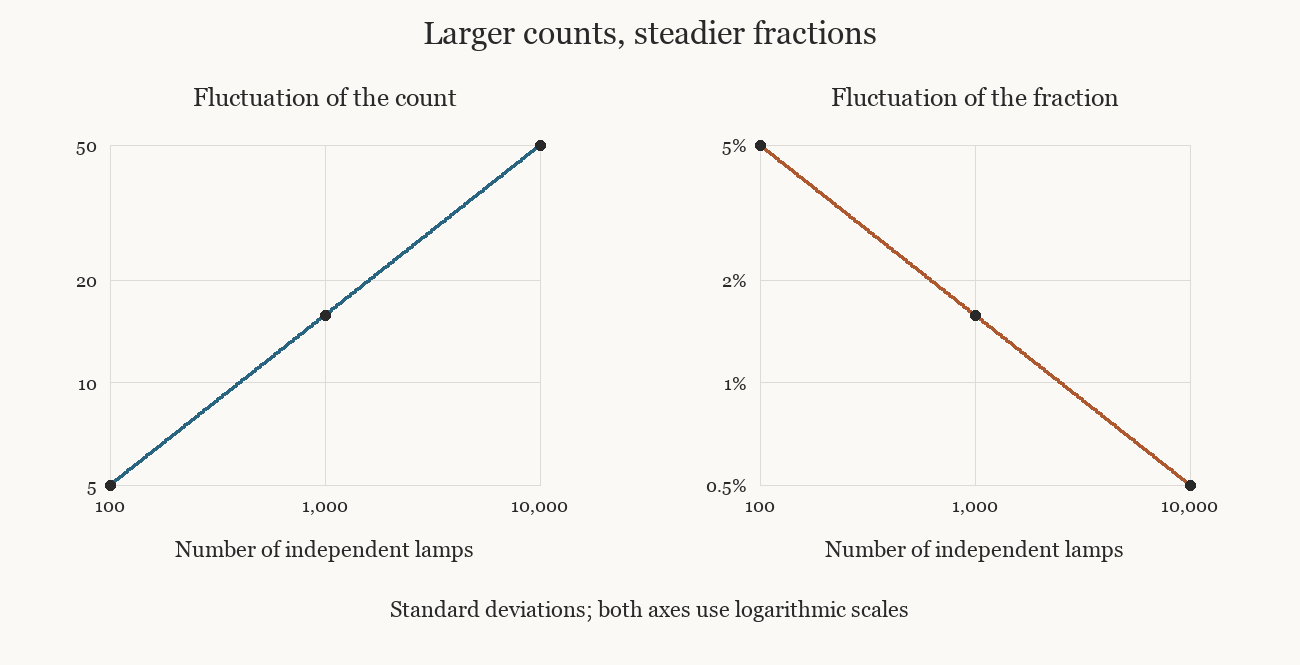
The left-hand graph follows the number of lamps by which the count typically varies; the right-hand graph divides that variation by the panel size. Both axes use logarithmic scales: equal distances correspond to equal ratios. Moving from one hundred to ten thousand independent lamps multiplies the count's standard deviation by ten and divides the fraction's standard deviation by ten.
Nothing in this argument forces a later switch to compensate for earlier outcomes. After an unusual excess of lights, every still-independent switch retains the same probabilities. The reduction concerns the distribution of the fraction over preparations of increasingly large panels. It does not introduce a correcting force into the switches.
Concentration and the shape of fluctuations
The shrinking variance lets us make a statement about probabilities. Choose a positive tolerance around the expected fraction one half. Whenever the observed fraction lies outside that tolerance, its squared departure is at least . Consequently, the average squared departure must be at least times the probability of being outside. Rearranging gives
This is an instance of Chebyshev's inequality. It bounds a probability using only a variance, so it need not be a close estimate. Its importance here is that, for any fixed tolerance, the upper bound tends to zero as grows. The fraction converges in probability to one half. We have obtained a law of large numbers for this model by following what independence does to the fluctuations.
There is a second question: what shape do the remaining fluctuations have? For the independent fair lamps, the exact count distribution is binomial. A count of occurs in as many equally likely configurations as there are ways to choose illuminated positions among . Counts near half the panel can be realized in many more ways than counts close to zero or .
For large , the central part of this distribution approaches a Gaussian bell when expressed in units of its own standard deviation. The variable
subtracts the expected count and divides the remaining departure by its characteristic size. Its distribution approaches a standard normal distribution, centred at zero with variance one. Roughly 68 per cent of outcomes then lie within one standard deviation and 95 per cent within two. These are approximate probabilities, not boundaries that outcomes cannot cross.
The central limit theorem explains this limiting shape for sums of independent, identically distributed contributions with finite, nonzero variance. The contributions need not be binary. It is a different statement from concentration: the law of large numbers describes the shrinking spread of an average, while the central limit theorem examines the shape visible after we magnify that spread. Neither statement warrants extending a Gaussian approximation without checking its accuracy far into the tails of a finite distribution. For this panel, exact binomial probabilities remain available when an unusually extreme count matters.
How correlations change the count
Return to the common switch. Two lamps always depart from their means in the same direction, so their product is always positive. The pair terms that cancelled under independence now reinforce the variance. There are many such terms: the number of distinct pairs grows approximately as the square of the number of lamps.
For variables with finite variances, the general rule is
Each sum adds the quantities indexed beneath it. The condition counts every distinct pair once. Covariance is the mean product of the two departures from their respective means. Positive covariance increases the variance of the total; negative covariance reduces it. Independence makes each covariance zero, although zero covariance alone does not generally establish independence.
For the common switch, every individual variance and every pair covariance equals one quarter. Adding them gives a count variance of . The illuminated fraction therefore has variance one quarter at every panel size. Increasing the number of lamps supplies more copies of the same random outcome, so the fraction never concentrates around one half.
Between the two extremes, divide the panel into groups of lamps. Each group shares one fair switch, and different groups switch independently. Assume is divisible by . There are independent groups, each contributing either zero or illuminated lamps. Adding their variances gives
With one hundred lamps in groups of ten, the standard deviation of the illuminated fraction is about 15.8 percentage points, compared with five for independent lamps. If group size stays fixed as the panel grows, the fraction still concentrates. If the entire panel remains one group, it does not. The number of independent groups determines the gain from making the panel larger.
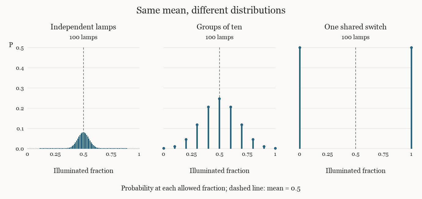
The dashed line marks the same mean in all three panels. Each vertical stem gives the probability of that particular fraction, so its height depends partly on how many different fractions are possible. The independent panel allows steps of one hundredth; groups of ten allow steps of one tenth; the shared switch allows only zero and one. The probabilities in each panel sum to one. The widening spread, rather than the height of the tallest stem, shows how much less representative the mean becomes.
What a steady average tells us
In a material, correlated regions rarely have the sharp boundaries of these wired groups. The covariance formula remains valid, and the dependence of correlations on distance determines how much their sum contributes. When correlations are short-ranged and their total contribution per site stays bounded as the system grows, the variance of a spatial average can still decrease in proportion to inverse system size. Long-ranged correlations can change that scaling. Near a continuous phase transition, treating a region as a collection of independent microscopic pieces can therefore miss precisely the fluctuations one hopes to explain.
The variance calculation also has a boundary of its own: it assumes finite second moments. Distributions with sufficiently heavy tails can violate that assumption, so the square-root scaling and the usual central limit theorem no longer follow. A finite mean can exist even when the variance is infinite; under independence and identical distributions, a law of large numbers can still apply if the absolute mean is finite. Concentration and Gaussian fluctuations should not be treated as an indivisible package.
For an actual measurement, we can test how the spread changes when we enlarge the observed region or collect additional samples. The independent-switch prediction is specific: multiplying the number of contributions by four halves the standard deviation of their average. A persistent departure invites examination of shared influences, long-lived correlations, changes in the preparation, or broad individual fluctuations. The mean remains useful, but the way its uncertainty changes with scale tells us whether it represents many independent contributions or a collective variation that averaging has failed to remove.
Letture collegate