When neighbours matter
Two arrows sit side by side on a screen. Each can point up or down. We record their orientations over many observations and find that each arrow points up half the time. These measurements tell us nothing about how often the arrows agree. They might move independently, remain almost always aligned, or tend to point in opposite directions. All three behaviours are compatible with the same statistics for either arrow considered alone.
We can build an interaction whose effects are small enough to calculate in full. At each tick, choose one of the two arrows at random. With probability , make it copy its neighbour. With probability , assign it a new orientation by tossing a fair coin. Leave the other arrow unchanged. Every random choice is fresh. This is a model of local copying with noise; interpreting the arrows as microscopic magnetic moments would require an additional physical argument.
How agreement accumulates
Copying always leaves the pair aligned. A fair reassignment produces agreement with probability one half, whatever the unchanged arrow is doing. Immediately after an update, the probability of agreement is therefore
For this particular two-arrow rule, that result holds after even one update. It does not mean that the full distribution has already settled. If both arrows initially point up, one update can produce a mixed pair, but cannot produce two downward arrows. Agreement alone leaves some of the state unresolved.
The same result can be obtained by following probability flows. An aligned pair becomes mixed only through a random reassignment that selects the opposite orientation, with probability . A mixed pair becomes aligned through copying or through the favourable half of random reassignments, with probability . Balancing the two flows gives
There is no preference for up over down in either process. For , random reassignments make every configuration accessible and allow it to remain unchanged. The four-state chain therefore has a unique stationary distribution. Reversing both arrows leaves the rule unchanged, so it must leave that distribution unchanged too. The two aligned configurations have equal probabilities, as do the two mixed ones:
With , each of the four configurations has probability one quarter. With , each aligned configuration has probability , while each mixed one has probability . Yet either arrow still points up with probability one half: for the first arrow, add the probabilities of up-up and up-down, obtaining .
The interaction has changed the joint behaviour without changing the distribution of either part. Looking only at the parts separately would miss its entire effect on these stationary probabilities.
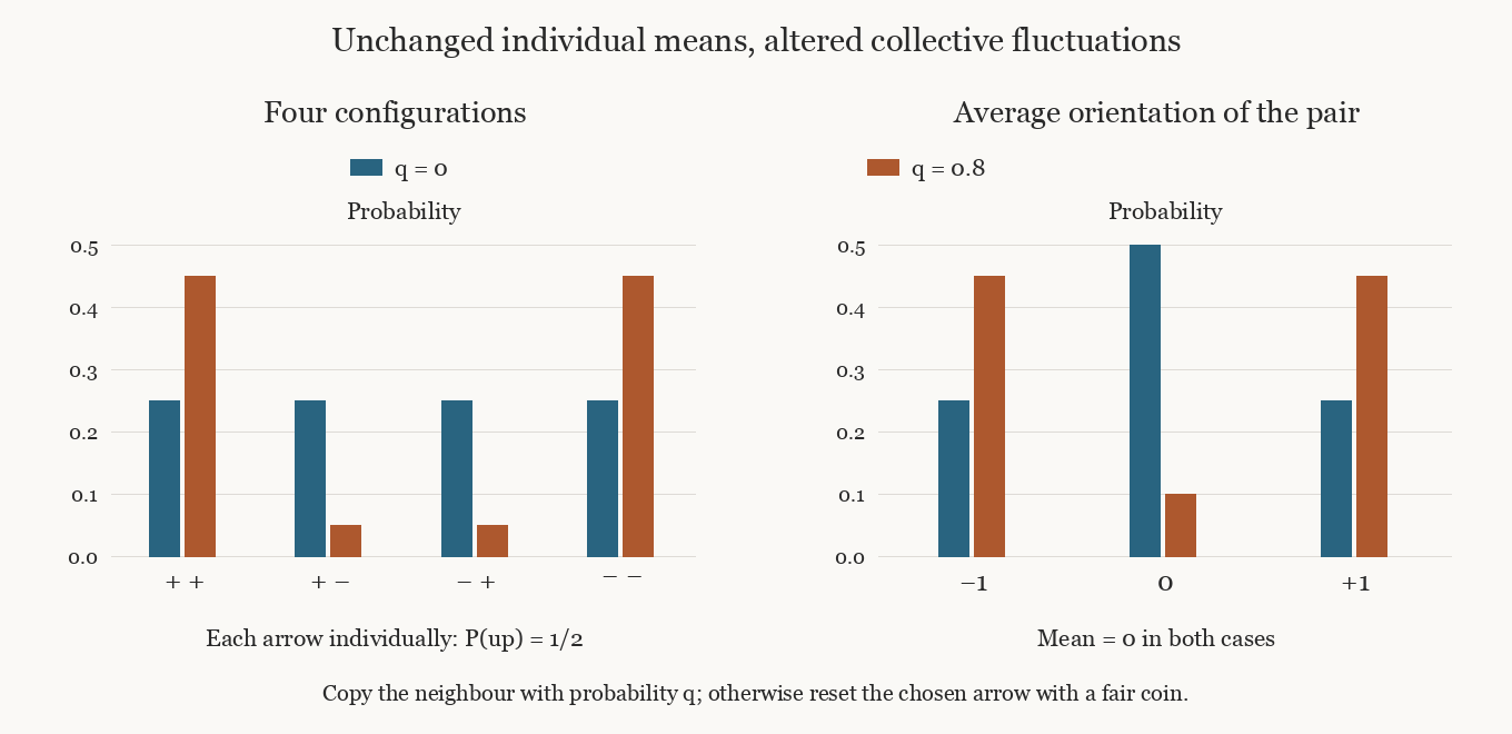
In the left panel, copying moves probability from the mixed configurations to the aligned ones. In the right panel, the same redistribution is expressed through the average orientation of the pair. The mean of that average stays zero, but its distribution becomes concentrated near the two extremes. A vanishing average orientation does not imply that a typical pair is internally balanced.
Measuring what one arrow tells us about the other
Assign the number to an upward arrow and to a downward one, calling their values and . Each has stationary mean zero. Their product is when they agree and when they disagree. Its mean is consequently
Angle brackets denote an average over the stationary probabilities. In this model, the mean product measures the preference for agreement directly. If the arrows were independent, their joint probabilities would be products of the individual ones and the mean product would be zero.
When individual means are nonzero, a raw product also contains agreement caused simply by those biases. Two independent arrows that each point up nine times out of ten will often agree. To isolate the dependence, subtract the product of the means:
This connected correlation, or covariance, is also the average product of the departures from each arrow's own mean. It measures whether those departures tend to occur together. Here the means vanish and the individual variances are one, so the covariance also equals the usual normalized correlation coefficient: . That equality of conventions is special to our chosen variables and distribution.
There is a more immediate way to read the dependence. Among stationary observations in which the first arrow points up, what fraction also have the second pointing up? Dividing the probability of up-up by the probability that the first arrow is up gives
At , seeing the first arrow up raises our probability for the second from to . The vertical bar means that we restrict attention to observations satisfying the condition on its right. No arrow has been changed by this calculation.
Why replacing a neighbour by its mean can fail
Let be the average orientation of the pair. Its possible values are , zero and . Its mean is zero for every , but squaring it before averaging retains the fluctuations:
The result follows by expanding and using . Independent arrows give a variance of one half. At , the variance is : the two contributions reinforce each other more often, so averaging them removes less of their variability.
Suppose we retained only the mean of each arrow and approximated their joint distribution by the product of their separate distributions. We would predict four equally likely configurations, regardless of . Both individual means would be exactly right, while the variance of would be wrong. This is the information discarded by a factorized description. Approximations that replace a fluctuating neighbourhood by an average face the same question: how much of the observable depends on the correlations they remove?
For a collection of many components, the variance of their sum includes every individual variance and every covariance between distinct pairs. Whether averaging suppresses fluctuations depends on how those pair contributions add up. Two arrows let us count the terms without approximation. A large system introduces the harder question of how far dependencies extend and how many pairs contribute appreciably.
At , random reassignments disappear. An initially mixed pair aligns at its first update, then remains frozen in whichever orientation won. Both aligned configurations are absorbing, and there is no longer a unique stationary distribution. The symmetric distribution approached as tends to one from below puts half its probability on each absorbing configuration. A single frozen pair cannot explore that mixture. This endpoint is a change in the allowed dynamics of a finite model; it is not evidence of a thermodynamic phase transition.
The same correlation from a different mechanism
The measured probabilities do not uniquely identify copying. Imagine another apparatus with no connection between the two arrows. Before each observation, a hidden controller independently chooses a signal or with equal probability. Each arrow then follows that signal with probability , and opposes it otherwise. Given the signal, the two choices are independent.
Each arrow again has mean zero. Its mean conditional on the signal is , so the mean product of the two arrows is . Choose
The resulting covariance is exactly . Symmetry then gives precisely the same four configuration probabilities as the copying apparatus. Even a complete catalogue of simultaneous pairs, collected at stationarity in the first apparatus, cannot distinguish these two mechanisms. Their time sequences may differ, because the controller in the second apparatus is redrawn independently before each observation.
An intervention offers another distinction. Hold the first arrow pointing up and allow only the second to update. In the copying apparatus, each update makes the second point up with probability . In the controller apparatus, fixing the first arrow changes neither the hidden signal nor the rule for the second, so the second still points up with probability one half. Merely observing the first arrow up gives in both models when ; forcing it up gives different predictions.
The distinction depends on specifying what the intervention changes. A real clamp might also disturb the environment, so its effects would have to be included in the model. For these two explicitly defined apparatuses, the comparison is exact: identical correlations arise from different mechanisms, and a controlled change separates them. The arrows' agreement tells us that their fluctuations belong in a joint description. Discovering why they agree requires a further experiment.
Letture collegate
Come lo scambio di energia definisce la temperatura e perché un reservoir finito produce il peso di Boltzmann.
7 min di letturaProbabilità stazionarie, tempi di mixing e limiti imposti dalle correlazioni a una lunga osservazione.
7 min di lettura