Moving through a space of theories
Heat a magnet sufficiently and it loses its spontaneous magnetization. The microscopic magnetic moments can still be present, but their collective orientation has changed. To study how such order disappears, we can use a deliberately restricted model: a square lattice with one arrow at each site, allowed to point either up or down. These two-state variables are called Ising spins. They retain the possibility of local alignment while leaving out the atomic structure of a real magnet.
Neighbouring arrows have lower interaction energy when they agree. The lattice exchanges energy with an environment held at temperature , so higher-energy arrangements also occur. At thermal equilibrium, a particular arrangement whose energy exceeds another's by has relative probability . Here , Boltzmann's constant, converts temperature into an energy scale. Increasing temperature brings this ratio closer to one: an energy difference becomes less decisive. The rule gives the probabilities of complete arrangements; the number of arrangements sharing a property also matters when we calculate that property's probability.
In the infinite square-lattice model with no applied field, spontaneous magnetization disappears continuously at a critical temperature. Near that temperature, regions of many sizes fluctuate together. Knowing an arrow's orientation tells us something about arrows well beyond its immediate neighbours, because the local interactions connect through the intervening lattice. A model that replaces each region by an independent average discards these correlations. We need a way to simplify the description while keeping the statistical relationships between regions.
A block is not yet a theory
Divide the lattice into square blocks, each three spins wide and three spins high. Replace the nine spins within a block by a single arrow pointing in the direction of their majority. Five upward spins and four downward spins produce an upward block arrow, as do eight upward spins and one downward spin. Since there are nine spins, a tie cannot occur. The resulting image has one arrow for each original block, and the distance between neighbouring arrows is three times the original lattice spacing.
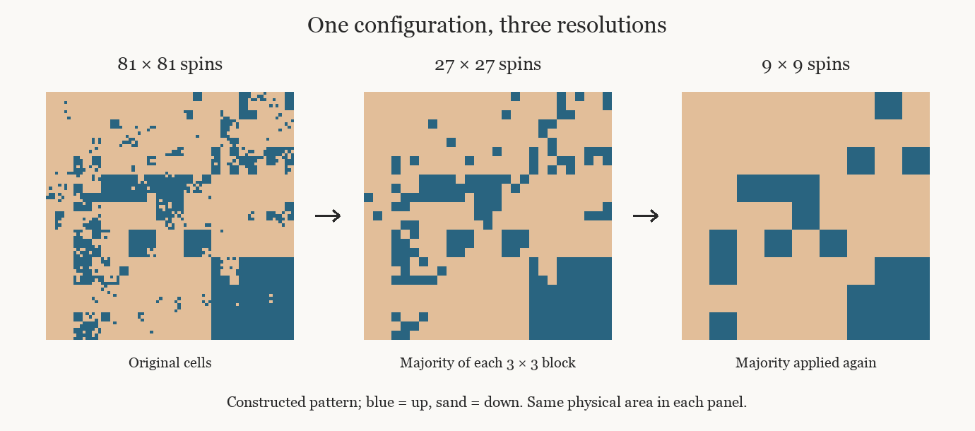
Each panel shows the same physical area, first with 81 cells along each side, then 27, then nine. The colours distinguish the two orientations. Small features disappear when their spins are outnumbered within a block; the next panel retains only the winning orientation. This configuration was constructed to illustrate the operation, rather than sampled from a magnet at thermal equilibrium. Its appearance therefore supplies no evidence of criticality or universality. Those properties concern the statistics of configurations and the transformation of their probability law.
This operation is a coarse-graining: several distinct microscopic configurations receive the same coarser description. An upward block arrow tells us that at least five of its original spins pointed upward, while leaving unresolved which ones they were. The loss of information is explicit enough that we can count it. Nine two-state spins admit configurations. Reversing every arrow pairs each upward-majority configuration with a downward-majority one, so 256 configurations produce each possible block arrow.
Counting them does not yet tell us their probabilities. A block with eight upward spins may have a different energy from a block with five, and the arrangement of the downward spins also matters because it changes the number of aligned neighbours. Spins along the edge of the block interact with spins in adjacent blocks. Consequently, the probabilities assigned to the microscopic configurations carry information both about the contents of a block and about its surroundings.
To obtain the probability of a particular coarse configuration, we must add the probabilities of every microscopic configuration that produces it. Suppose two neighbouring block arrows both point upward. There are many microscopic ways of obtaining that pair, and each has its own probability under the original model. Their total is the probability that the coarser description must assign to the pair. The same procedure applies to an entire coarse lattice. Once its block arrows have been specified, we collect all compatible microscopic configurations and sum their probabilities.
This gives the new description a precise obligation. It must reproduce the probabilities of the block variables defined by our rule. Drawing larger arrows achieves only the change of variables; the calculation of their joint probabilities supplies the statistical model those arrows obey. We can then ask whether that model can be expressed through effective interactions, just as the original model expressed probabilities through the energies associated with neighbouring spins and the temperature of the environment.
The coordinates of a theory
In general, the effective interactions differ from the original ones. Even if individual spins interacted only with their nearest neighbours, the block variables can acquire interactions extending farther across the lattice, or involving several blocks at once. Summing over the unresolved spins carries their effects into the probabilities of the variables we retained. If we force the resulting model to contain only one nearest-neighbour coupling, we are making an approximation whose adequacy needs to be checked.
It is useful to think of the model as having a set of adjustable parameters. One controls the preference for alignment between nearest neighbours. Another could control an interaction between more distant spins. An applied field introduces a preference for upward rather than downward orientation. For a thermal model these quantities can be expressed in dimensionless form, comparing the relevant energies with the thermal energy scale , where is temperature. A value for each parameter specifies a particular statistical model.
With one adjustable parameter, all its possible values can be placed along a line. With two, a pair of numbers specifies a point on a plane. Allowing additional interactions supplies further coordinates, whether or not we can draw the resulting space. We call this a space of theories because each point specifies a set of rules for assigning probabilities, rather than a single configuration of spins. A point in phase space describes a possible state of a system. A point in theory space describes the model according to which those states are weighted.
Coarse-graining carries us from one such model to another, but a comparison between them requires one more adjustment. The new lattice spacing is three times as large. If we now use that spacing as our unit of length, neighbouring block arrows are once again one unit apart, just as neighbouring original spins were before. Other retained variables may also require a change of normalization when their magnitudes are compared. We can then compare the forms and dimensionless parameters of the two descriptions on the same footing.
The combination of coarse-graining and rescaling is a renormalization transformation. Repeating it generates a sequence of effective models, called a renormalization flow. Each step represents larger physical regions through the elementary variables of the description. We could perform the entire calculation on an equilibrium probability distribution at one fixed temperature: the flow records increasing scale, with no passage of physical time required.
This differs from omitting velocity in a strongly damped mechanical system because it relaxes quickly. Here we sum over unresolved spin arrangements to obtain equilibrium probabilities. That operation does not require the discarded spins to move faster than the retained variables. Predicting how the block arrows change in time would be a further problem; an accurate equilibrium distribution alone does not specify their dynamics.
Flows and fixed points
Some models can be reproduced by the transformation. After coarse-graining and restoring the units, their dimensionless descriptions have the same form and parameters as before. Such a model is a fixed point. The condition refers to the statistical description, so it does not require a snapshot to reproduce the position of every cluster when magnified. Different snapshots can look different while their distributions of fluctuations obey the same scale-dependent relations.
To measure the range of a statistical relationship, imagine sampling many equilibrium configurations and comparing two sites. We record how each spin departs from its own mean orientation, multiply those departures and average the product. A positive result means that departures in the same direction occur more strongly than independence would predict. This is a connected correlation. Subtracting the means removes the agreement already explained by an overall magnetization.
The correlation length characterizes how far these correlations extend. In the disordered phase away from the transition, they decay at long distances with an exponential cutoff. The correlation length sets that decay scale; it is not a sharp boundary beyond which dependence suddenly vanishes. As criticality is approached, it grows. Expressing a given physical length in units of blocks three times wider divides its numerical value by three.
At an ordinary scale-invariant critical fixed point, the correlation length is infinite in the idealization of an infinite system. Dividing it by any finite scale factor does not produce a finite range. This permits nontrivial correlations to survive repeated changes of scale. In a finite sample, the size of the sample limits the range over which this behaviour can be observed; the microscopic lattice spacing also remains a lower cutoff. Critical scale invariance concerns the behaviour between the relevant cutoffs and its limiting description.
A physical model tuned to a critical point need not already be the fixed-point model. Its short-distance interactions can still change under coarse-graining. In the cases described by an ordinary critical fixed point, successive transformations bring its long-distance description toward that point as the influence of certain microscopic differences diminishes. Reaching the critical conditions and starting exactly at a renormalization fixed point are therefore distinct statements.
To understand what can diminish and what can grow, imagine a simplified map with two coordinates, and . Both measure departures from the fixed point, which lies at zero for each. We choose a transformation that halves and doubles at every step:
These factors are chosen to make the geometry easy to follow. They have not been calculated for the square-lattice magnet. The coordinate represents the role of a deviation from critical conditions, while represents a deviation that the transformation suppresses. In a real calculation, suitable coordinates can combine several of the original interaction parameters, and the factors multiplying them have to be determined from the transformation itself.
Start at and . Successive steps give , then , then , while remains zero. The points approach the origin. Starting with a different value of changes the early part of this sequence but leads to the same destination. Along this direction, the description progressively loses sensitivity to its initial difference from the fixed point. We call such a perturbation irrelevant, referring specifically to its diminishing size under the transformation near that fixed point.
Now start at the same value of , but let . The first coordinate still shrinks, while the second becomes , then , then . For several steps the point may appear to approach the origin, because the shrinking coordinate initially dominates its distance. Eventually the growing coordinate carries it away. This perturbation is relevant: a small initial difference becomes increasingly important as we pass to larger scales.
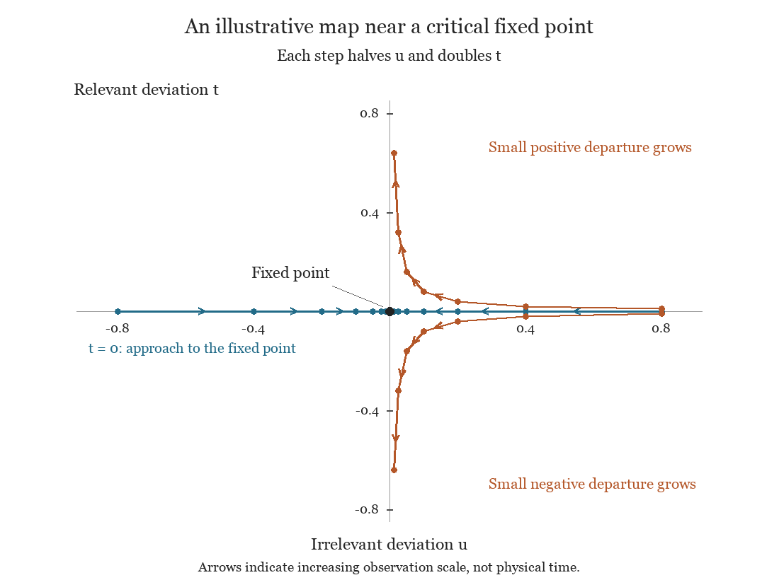
The points follow the illustrative rule , . On the line , successive transformations approach the fixed point. A small positive or negative initial value of eventually carries the sequence away, although continues to decrease. The coordinates measure deviations in theory space; the arrows indicate increasing scale, and the numerical factors are chosen for this example.
The fixed point attracts trajectories along one direction and repels them along the other. This geometry explains why critical behaviour usually requires adjustment. In the example, we must set to zero to keep the growing departure absent. For the usual ferromagnetic Ising critical point, temperature and the symmetry-breaking field provide relevant adjustments, while other microscopic perturbations can shrink once those conditions have been imposed. A generic sample at a generic temperature does not flow toward the critical fixed point indefinitely.
Critical surfaces and shared behaviour
The set of models that do approach a given critical fixed point forms its critical surface, more precisely its stable set in this description. In our two-coordinate illustration it is just the line . A basin of attraction refers to the set of starting points that reach an attractor under repeated transformations; at a critical saddle, convergence is restricted by the relevant directions. Treating the critical point as the bottom of a basin that attracts every nearby model would erase the need to tune the system, which is one of the physical facts the geometry must explain.
This distinction also gives a way to understand approximate critical behaviour. A model with a very small relevant departure can remain near the fixed point for many transformations before moving away. Each step represents a larger block of the original system, so spending many steps in that neighbourhood corresponds to a broad interval of scales displaying approximately critical behaviour. A larger initial departure leaves the neighbourhood sooner and produces a smaller interval.
The numerical example allows us to follow this relation without solving a differential equation. Starting with , six doublings bring it to one. Starting with takes seven. If each transformation combines lengths by a factor of three, the second starting point remains near criticality for one additional step and reaches a length scale three times larger. The values one and three here belong to the chosen illustration: one marks our reference departure, and three is the blocking factor. In a physical model, the corresponding growth factor determines how the characteristic correlation length increases as critical conditions are approached.
The mechanism behind a scaling law is visible in this comparison. Reducing the initial departure by a fixed factor adds a fixed number of renormalization steps; each additional step multiplies the length represented by a fixed amount. Repeating the procedure links successive multiplicative changes in departure to successive multiplicative changes in length, which is the structure of a power law. Calculating its exponent requires the actual growth factor of the physical transformation. The illustration explains where that factor enters, while leaving its model-specific calculation open.
We can now consider two microscopic models with different short-distance interactions. If, after their relevant parameters have been tuned, their renormalization flows approach the same critical fixed point, the large-scale behaviour governed by that point can agree. In the standard setting this includes critical exponents and appropriately normalized scaling functions. Their critical temperatures can still differ, as can the amplitudes that convert a universal relation into the units of a particular experiment. A shared universality class is a statement about specified asymptotic behaviour, with these distinctions retained.
Which fixed point governs a model depends on more than its superficial resemblance to another. Spatial dimension, the symmetry of the order parameter and the range of interactions can alter the outcome; additional constraints matter when the question concerns dynamics. There are also perturbations called marginal, whose leading change neither shrinks nor grows, and whose eventual effect requires examining the transformation more closely. The two-coordinate map leaves those cases out so that the meaning of attraction and repulsion can be established without confusing it with a classification of every possible flow.
What the flow can test
Suppose two microscopic models reproduce a material's average magnetization at one temperature. They may still predict different correlations between distant regions. Measuring those correlations across distances and temperatures tests more than the single average. Near a continuous transition, the growth of the correlation length and the shapes of correlation curves provide quantitative consequences against which a proposed large-scale description can be checked.
There is also a direct test of the coarse-graining itself. Generate configurations from the microscopic model, replace each block by its majority arrow, and measure the resulting block statistics. An approximate effective model should reproduce the statistics it claims to retain. If it gets the average orientation right but misses correlations between blocks, the agreement of the averages cannot justify it. An interaction omitted from the effective model may still matter at the scale being examined. Following the discrepancy across successive blocking steps helps distinguish a short-distance correction that fades from a difference that continues to grow.
Letture collegate