Moving Across Theories
On statistical mechanics and why science works
Introduction & Entropy
Statistical mechanics is a fundamental branch of theoretical physics which explains how macroscopic quantities emerge from microscopic ones. It was born at the crossroads between XIX and XX Century and it was first conceived to formalize and establish how common physical quantities (such as temperature) are deduced from microscopic features (such as velocity) of each particle of the gas.
The first relevant results come from Maxwell (1859), who managed to derive the temperature and energy of an ideal gas through a probability distribution of the velocity of the particles of the gas, and Boltzmann, who formalized the relation between all the microstates of a system and the entropy of it:
Sticking to the case of the ideal gas, we can define a microstate as a particular set of configurations for all the particles of the gas (e.g. a configuration where all the particles have the exact same velocity is one microstate, if we increase the velocity of just one particle we obtain a new and different microstate for our system). The Ω in the formula above stands for the number of microstates that are compatible with a certain macrostate.
Entropy is a fundamental property of any system, as well as of our universe itself. Its proper definition depends on the field of study; it is commonly referred to as the measurement of disorder, but I personally like to define entropy here as the uncertainty we have on the possible microstates when we just know a specific macroscopic state.
Boltzmann made one of the most remarkable discoveries in the history of science, writing an explicit relation between the microscopic world and the macroscopic one. Moreover, this is the first time we can see how the concept of information has a direct impact on reality itself.
We need to dig a bit into the details of Boltzmann’s work to fully understand what’s coming next. Also, the relevance and the impact of this breakthrough needs to be explained more in detail anyway.
Let’s pick the simplest system you can think of: two particles, two possible states per particle. Here, for the sake of argument, let’s forget about the real meaning of “state”: it’s just an abstract tag assigned to the particle, and this tag can have two values in this simple example. The number of microstates will be calculated as (number of microstates per particle) ^ (number of particles) = 2^2 = 4.
Two questions arise:
- What is the entropy of this system?
- How can we understand in which state is each particle?
The answer to the second question will bring us to the evaluation of the entropy. So let’s start by calling the microstates with their names: A and B (we’re being creative here). The four configurations the system allows are:
If we do not know which microstate the system is actually in, the best we can do is assign a probability to each possible microstate.* For this scenario, let’s assume a uniform probability to each state:
Now, let’s come back to our goal of finding the value of entropy, by defining a “macrostate” in this toy model: “how many particles are in state A”:

Let’s take a look at the table:
- The macrostate where 2 particles are in state A can be realized in just one arrangement, so we don’t have any uncertainty about the microstate (S = 0)
- Same for the macrostate with 0 particles in state A (S = 0)
- The macrostate with one particle in state A can be realized in two ways, so we still have uncertainty about the microstate that resulted in that macrostate (S > 0)
Now that we have evaluated the possible values of entropy in this simple case, let’s get back to the ideal gas. The construction of two particles-two states can be generalized: each particle can be fully identified by its position and velocity, so instead of having a single variable (what we called “tag” before) with two possible values, we have:
Where the first three are the coordinates of the particle, while the last are the components of the velocity of the particle, decomposed along the three Cartesian axes. A particle state is now defined by 6 variables. Moreover, the particle can assume any position and any velocity in principle, so this means that instead of having just two possible values for the state, we have infinite possible values. We cannot simply count the number of microstates; we need to introduce the concept of volume.
Let’s simplify again the situation here, let’s concentrate on a single particle moving on a single line, of length L. It’s clear it can assume infinite positions between 0 and L, but we may say that the set of positions the particle can assume is a line of length L.
In the same way, if we constrain the particle to live inside a box with faces of side L, we can identify a volume in which you can find the state of the particle.
We can apply the same argument to the velocity: here, instead of having a volume in the real world, we need to imagine a volume in the space of velocity.
The space containing all possible microstates of a particle (all possible positions and velocities of that particle) is called the phase space, of dimension 6. For an ideal gas composed of N particles, we have a phase space of 6N dimensions.
Therefore, a macrostate can be identified as a region containing all the microstates that look identical at the macroscopic level. Now, let’s get to where things get really interesting. Statistical mechanics of course finds applications outside the description of the ideal gas. Scientists have modeled several microscopic systems, in a wide range of conditions, finding out remarkable behaviors in critical ones.
Critical Phenomena
This discussion, so far, is relying on the concept of emergence of macroscopic quantities from microscopic features. The implicit assumption in this framework is that the effect of these microscopical interactions will result in a uniform average that we can measure as a macroscopic quantity. Zooming out of the particle realm feels like blurring all the details and getting a uniform behavior out of it. This is acceptable for most cases, where a lot of microstates produce the same macroscopic behavior (this means entropy can be considered high if we follow the previous discussion). This is not always the case.
There are particular conditions in which the simple idea of zooming out, averaging microscopic fluctuations and obtaining a smooth macroscopic behavior starts to become problematic. One of the most famous examples comes from magnetism, where some materials are able to develop a spontaneous magnetization below a certain temperature, while above it they completely lose this property. The temperature at which this transition happens is called the critical temperature.
To understand why this case is so peculiar, physicists introduced simplified models able to isolate the essential ingredients of the problem. One of the most famous examples is the Ising model, which we can imagine as a regular grid (let’s imagine this in two dimensions for now, for simplicity of visualization) where each point contains a variable that can assume only two possible values, conventionally represented as an arrow pointing either up or down:
↑ ↓
These variables are called spins. Their actual physical meaning is not particularly relevant for us at this stage: for the sake of the argument, we can treat them exactly as the A and B tags introduced before. The only important additional assumption is that neighboring spins interact with each other, with configurations where nearby spins are aligned being energetically favored with respect to configurations where they point in opposite directions.
At low temperature, this tendency to align dominates over thermal fluctuations and large portions of the system tend to organize in the same direction. At high temperature, thermal agitation becomes dominant and spins are much more randomly distributed. If we stop here, this seems to fit perfectly with what we discussed before: microscopic fluctuations exist, but when we look at the system from far enough away they average out and leave us with a relatively simple macroscopic behavior.
Close to the critical temperature, though, the system develops fluctuations on increasingly large scales. Small regions of aligned spins appear inside larger regions, which can themselves be part of even larger structures. There is no longer an obvious size that characterizes these fluctuations, and this is the first signal that our simple idea of “microscopic details disappear when we zoom out” needs to be refined.
To make this statement more precise, we need to introduce the concept of correlation. Suppose we pick one spin in our lattice and then look at another one placed at some distance from it. We can ask:
How much knowing the state of the first spin tells us about the state of the second one?
If the two spins are very close, we expect the answer to be “quite a lot”, since neighboring spins interact and therefore their configurations are not completely independent. If we move sufficiently far away, however, under ordinary conditions the information carried by the first spin becomes progressively less useful for predicting the second one. The quantity that describes this behavior is called the correlation function. Leaving all the exact mathematical definitions behind: what matters is that it tells us how strongly two regions of a system are related as a function of the distance between them. Under normal conditions, correlations decay with distance. After some characteristic scale, two sufficiently distant regions behave almost independently of each other. This characteristic distance is called the correlation length and is usually indicated by ξ. We can think of ξ as the typical distance after which one region of the system has essentially “forgotten” what another region is doing.
At this point, we can provide a physical explanation for the averaging procedure we have been implicitly using since the beginning. If correlations extend only over a finite distance, we can divide a very large system into regions that are approximately independent of each other. When we zoom out, the local fluctuations occurring inside these regions tend to average out, while only a much smaller amount of information survives at the macroscopic level. Around a critical point, however, something very different happens. As the system approaches the critical temperature, the correlation length becomes larger and larger, until, in the idealized limit of the critical point, we can write:
This does not mean that our physical sample has suddenly become infinite. It means that there is no longer a finite characteristic length (typically the distance between atoms in the grid) beyond which correlations can safely be neglected. Fluctuations can now exist over microscopic distances, intermediate distances and macroscopic distances at the same time: there is no privileged scale anymore.
This property is called scale invariance, and it introduces a very interesting problem: if structures exist at every scale, how can we decide which microscopic details should be averaged out to extract the macroscopic quantities we’re interested in?
As you can guess, close to a critical point, jumping directly from the smallest scale to the largest one becomes dangerous because important structures may exist at every intermediate scale. Instead of averaging everything at once, we can therefore try to zoom out gradually, removing only a fraction of the microscopic information at every step. This procedure is called coarse-graining. Let’s get back to the Ising model. Imagine dividing the original lattice into small blocks, for example groups of neighboring spins, and replacing every block with a single effective spin representing the behavior of the group. A very simple rule could be to assign the effective spin according to the majority of the spins inside the block: if most of them point up, the new spin points up; if most of them point down, the new spin points down. By doing this, we have clearly lost information. Looking only at the effective spin, we can no longer reconstruct the exact microscopic configuration of the original block: the point of this is to extract the information we need from all spatial scales at which the correlation function operates: at each scale, components (we cannot call them just particles anymore, since we have already aggregated them in the first coarse-graining step) contribute with interactions to the evaluation of the final macroscopic quantity. In the standard situation, the scale is just the microscopic/particle scale.
After one coarse-graining step, our original lattice has become a smaller lattice composed of effective spins. We can now apply the same procedure again, grouping these effective spins into larger blocks and replacing them with new effective variables. Then we can repeat it again and again. There is an important disclaimer to reflect on: the effective system we obtain after coarse-graining is not exactly described by the same numerical parameters as the original one. Let’s say, for simplicity, that the strength of the interaction between neighboring spins is represented by a parameter K. Before coarse-graining, our model is characterized by a certain value of K. After replacing groups of spins with effective spins, the interaction between these new variables will in general have a different effective strength, which we can call K′. So, we can say that K → K′; if we apply coarse-graining again, K′ → K″, and so on.
The process generates a sequence:
Let’s try to generalize by adding a generic number of parameters (which is realistic, since the Ising model is just a toy model). In the simplest possible example, suppose there is only one parameter K. All the possible values of K can then be arranged along a line, and every point on that line represents a slightly different version of our theory. More generally, with N parameters we obtain an N-dimensional space: this is called parameter space, or, in a more general language, theory space.
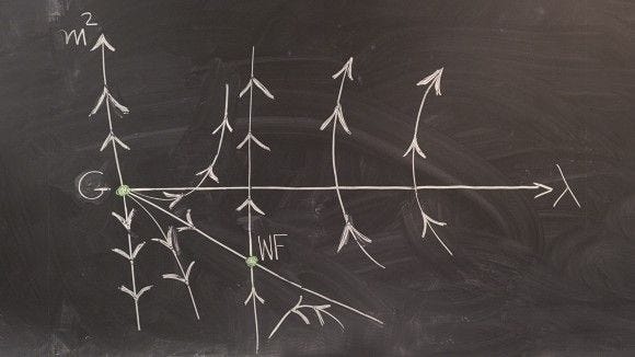
A point in phase space represents a possible state of the physical system; a point in parameter space represents a possible theory used to describe the system. The process of coarse-graining moves us from one point of this parameter space to another, which means that zooming out is equivalent to moving across different theories. The flow inside theory space is called renormalization.
A renormalization transformation takes a theory defined at a certain scale, removes some microscopic degrees of freedom through coarse-graining, changes the scale of observation and produces a new effective theory describing the same system at a larger scale. Symbolically, in our one-parameter example, we can write:
where R represents the renormalization transformation. We can think of R as a machine. We give it a theory characterized by K; it performs the coarse-graining procedure and returns a new theory characterized by K′. We can then feed this new theory into the same machine again, obtaining K″, and continue indefinitely.
The natural question therefore becomes: where do we get to after repeating this operation many times?
Among all the possible points in parameter space, there can be special points where the theory stops moving. Suppose we start from a particular value K*. After applying the renormalization transformation, we obtain exactly the same value:
K* will be called a fixed point. The physical meaning of this condition is quite remarkable. If a theory sits at a fixed point, changing the scale at which we observe the system does not change its effective description: zooming in or out does not change the model we use to describe the system: this clearly reminds us of what happened at the critical point.
This dump of information you just received is not pointless: from this point we can introduce one of the most remarkable conceptual achievement in natural science that is the concept of universality: let’s take into account several different theories, theories that may even have different microscopic quantities or interactions, if they eventually end up in the same fixed point, after the renormalization, they will result in the same theory at the critical point: we observe the same behavior out of systems that look completely different underneath. If this happens, we say the systems belong to the same universality class.
The concept of universality brings us to another consequence of the renormalization framework which, in my opinion, is even more relevant than the mathematical procedure itself: the idea that a theory does not necessarily need to describe every possible scale of reality in order to be useful; indeed, it turns out it is always the opposite: effective theories, theories that are built to describe a system inside a certain range of scales, deliberately ignore degrees of freedom which are not relevant inside that range. This may sound strange at first, because we usually tend to associate a “better” theory with a theory that contains more information. For example, if quantum mechanics gives us a deeper description of matter than classical mechanics, why should we ever use Newton’s equations again? The answer is simply that, if we want to calculate the trajectory of a football, describing the quantum state of every atom composing it would not make our prediction more useful: it would just introduce an insane amount of information which has essentially no impact on the phenomenon we are interested in.
The same happens at basically every level of physics: every time we change scale, we change the models and frameworks we use to describe reality. This means that a theory describing a deeper level of reality does not necessarily contain a “more correct” or “complete” description of the phenomena we observe at every scale: it contains more microscopic information, which is a different thing.
We can now close the discussion on the concept of information we introduced at the beginning: the declared goal of statistical mechanics was to derive macroscopic quantities from microscopic features, and the reality is that in doing so we have a procedure that tells us what information can be cut moving across different physical scales and why. It is also why universality itself is conceptually inevitable: relevant parameters survive the process and become important at larger scales, while irrelevant parameters slowly disappear from the effective description. So, after spending half of this article building increasingly detailed descriptions of microscopic states, we ended up finding out that a large part of those details may not matter at all for the macroscopic behavior we are trying to explain. Which is quite funny, but ironically, the point of the discussion.
The incredible machinery of renormalization asks a question that basically appears almost everywhere: if a system contains an enormous amount of information (which every real system does), which part of that information is actually necessary to describe its behavior at the scale we care about? Moreover, I think this mathematical technology is the most convincing explanation we have of why our incredible models, therefore the scientific method itself, actually work when compared with reality. Apparently, we always managed to coarse-grain reality with our intuition till this very moment. Maybe it’s time for us to step up and do this on purpose, at scale, as a new scientific and academic manifesto.
* For us, it’s trivial to think of probability as the parameter to decide, but for scientists at that time, this was a huge leap ahead: during the previous centuries, science was backed by the Determinism Principle, a philosophical belief that all events are determined completely by previously existing causes. As of now, we know that this is not possible due to quantum mechanics constraints, but this discussion still holds if we neglect quantum effects: solving the motion equations, which determine the trajectory in space and the velocity in any future moment with absolute precision, would be impossible for a gas which is made of, let’s say, ~10^23 particles; it would take millions of years, even with contemporary technology. We need to come up with something else.
Letture collegate