How many ways can the same thing happen?
Imagine a container divided into two equal chambers, with a door in the partition between them. We put a gas in the left chamber, leave the right one empty, and open the door. Molecules can now cross the partition, and after a while the gas occupies both chambers. If we keep watching, the amount of gas on either side remains close to half the total, although individual molecules continue to pass through the opening. The visible result is steady enough that we can stop paying attention to it, while the motion producing that result continues without interruption.
This is a familiar event, but explaining it requires some care. A molecule crossing from right to left obeys the same physical laws as one crossing from left to right. Nothing in the open doorway prevents the gas from returning to the chamber where it started. Yet a container of gas does not ordinarily empty one of its chambers by itself. To understand what makes the two situations so different, we need to look more closely at what we mean when we say that the gas is in a particular state.
We can begin with a smaller description, one that we can hold entirely in view. Suppose there are four particles, which we label so that we can tell them apart, and suppose the only thing we record about each particle is whether it is in the left chamber or the right one. We write these possibilities as A and B. The string AABB means that particles one and two are on the left, while particles three and four are on the right. ABAB describes a different arrangement, even though it puts the same number of particles in each chamber.
For this small model, a complete assignment of the four labels is a microstate. The word refers to the most detailed description admitted by the model. Here we have deliberately left out the positions and velocities of the particles within each chamber; those details would be needed for a microscopic description of an actual gas. Our reduced description lets us isolate a question that can be answered before we consider their motion: how many arrangements produce the same result when we count the particles on the left?
The answer depends on what that count tells us. If it is four, we know that the arrangement is AAAA. If it is zero, we know that it is BBBB. If it is two, there are several possibilities: AABB, ABAB, ABBA, BAAB, BABA and BBAA. Each of these gives the same reading to an instrument that counts particles in the left chamber. We call that reading a macrostate, and in this example it leaves six possible microstates unresolved.
The distinction is a consequence of the question being asked. An instrument that reports which particle is in which chamber distinguishes all six arrangements. An instrument that reports only how many are on the left treats them as equivalent. Once we have chosen the macroscopic measurement, we can group together all the microstates that agree with it. A macrostate is then represented by an entire group of microscopic possibilities.
There are sixteen arrangements altogether. To see why, start with the first particle, which has two possible labels. For each of those possibilities, the second particle can also be A or B, giving four pairs. Adding the third doubles the number again, and adding the fourth brings it to sixteen. The compact notation for this repeated multiplication is . The exponent, four, records how many particles each contribute a choice between two alternatives.
The sixteen possibilities are distributed unevenly among the five possible macroscopic readings. There is one arrangement with no particles on the left, four with one, six with two, four with three, and one with four. We have obtained this difference by counting, without making any assumption about forces or motion. Having two particles on either side can happen in six different ways; having all four on a specified side can happen in only one.
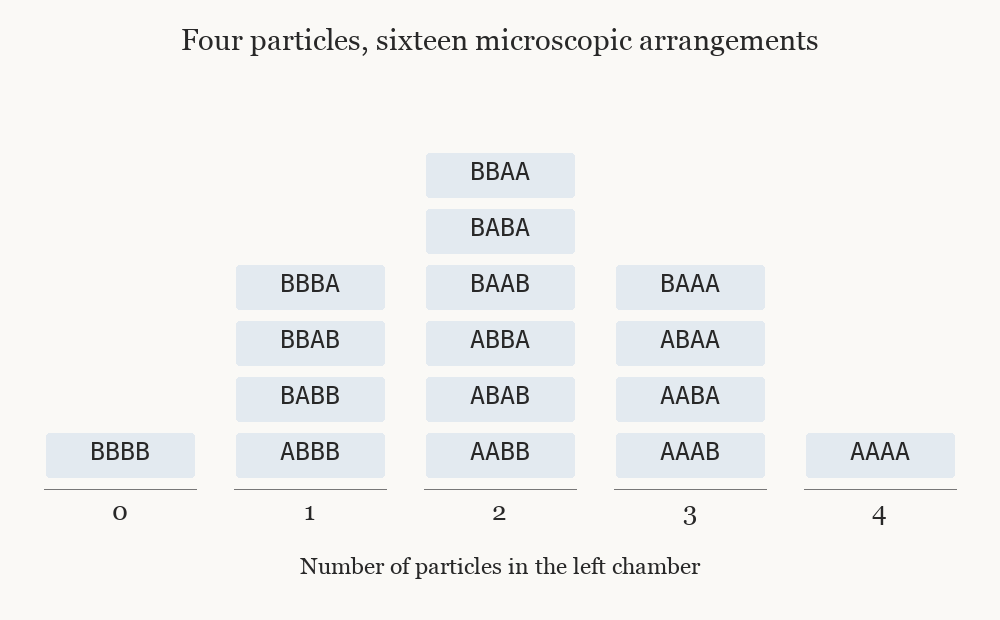
Each string retains the identities of the four particles. Reading up a column changes their arrangement while preserving the count below it. The different column heights are the multiplicities we have just calculated; they become probabilities only after we specify how the strings are sampled.
To turn this count into a statement about probability, we need an additional assumption. Suppose that each particle is equally likely to be on either side, and that learning which side contains one particle gives us no information about the others. Under these conditions, all sixteen arrangements have equal probability. Each receives one sixteenth of the total, so the probability of observing two particles on the left is six sixteenths. The probability of finding all four on the left is one sixteenth. Equal probabilities at the microscopic level have produced unequal probabilities for the macroscopic readings.
The assumption matters. We could install a device that always moves the four particles together, allowing only AAAA and BBBB. The other strings would still be available in our written description, but the device would never produce them. If the device spends half its time in AAAA and half in BBBB, each particle is still on the left half the time. Looking at one particle at a time would therefore give the same probabilities as before. The difference appears when we look at the particles together: finding one on the left now tells us where all the others are. Equal probabilities for individual particles do not establish independence. A count of possible configurations becomes predictive only when we know which configurations the system can access and how they are weighted. In the independent, equally likely model, the weighting is particularly simple, which is why it makes a useful starting point.
We can extend the counting procedure without writing down every string. To obtain two A labels with five particles, the fifth particle can be A, in which case the first four must contain one A, or it can be B, in which case the first four must contain two. There are four arrangements of the first kind and six of the second, giving ten in all. Adding the corresponding counts in this way constructs the possibilities for five particles from those for four, and repeating the operation carries the calculation to any larger number.
Suppose we increase the number of particles while keeping the independence and equal probabilities assumed above. With one hundred particles there are arrangements, a number obtained by doubling one hundred times. Only one of them places every particle on the left. Its probability is therefore one divided by , approximately one chance in a million million million million million. The arrangements with particles distributed across both chambers occupy almost all the remaining possibilities.
Even here, however, finding exactly fifty particles on the left is only about an eight per cent event. That may seem at odds with the claim that a gas settles near an even division, until we notice what the claim actually requires. Counts of forty-nine and fifty-one also describe a nearly even division, as do many nearby readings. If we include every count from forty to sixty, the probability is about ninety-six per cent. These figures follow from the same counting procedure used for four particles, extended to the longer strings. The stable macroscopic appearance belongs to a range of nearby readings, each supported by many microscopic arrangements.
In the independent-particle model, increasing the number of particles concentrates an increasing share of the probability within any fixed fractional tolerance around an even division. For a large dilute gas at equilibrium, away from conditions where long-range correlations matter, the relative fluctuations can likewise become too small to distinguish with an ordinary instrument. A macroscopic instrument can consequently return the same reading while the particles keep exchanging places and the microscopic configuration keeps changing. What looks stationary at one level of description can contain extensive motion at another. The number of configurations compatible with a macroscopic reading gives us a way to make that difference quantitative.
Let us call this number , the Greek letter omega. For the four-particle model, is six when the left-hand count is two, and one when the count is four. We would like a quantity that records this multiplicity while remaining useful when systems become large. Counting directly quickly produces enormous numbers, and it has another feature worth considering: when we combine independent systems, their numbers of possibilities multiply.
Suppose one container has four compatible arrangements and another has eight. If every arrangement in the first can coexist with every arrangement in the second, the combined description admits thirty-two possibilities. Four times eight gives thirty-two. A measure that added when independent systems were combined would be easier to connect to the additive quantities used in thermodynamics. We can construct one by asking how many doublings are needed to obtain the number of possibilities.
Four is reached after two doublings from one, eight after three, and thirty-two after five. Combining the containers has therefore added their numbers of doublings: two plus three gives five. The function that assigns these values is called the logarithm to base two, written . It can also assign intermediate values; six lies between four and eight, so lies between two and three, at approximately 2.585. A logarithm allows us to express multiplicity on a scale where multiplication becomes addition.
In thermodynamics the conventional formula uses a closely related logarithm, the natural logarithm, written . Changing from to multiplies every answer by the same constant, just as changing the unit of a length changes its numerical value without changing the length being compared. Boltzmann's entropy of a macrostate is written
Here denotes the entropy, and , Boltzmann's constant, supplies the physical units of joules per kelvin. The logarithm carries the dependence on the number of compatible microstates. In the four-particle model, the macrostate with all particles on the left has , giving zero on this counting scale, whereas the macrostate with two particles on the left has entropy . The zero refers to the alternatives represented in our model; it does not imply that the molecules of a real gas have no other contributions to their thermodynamic entropy.
This definition also explains a useful connection with uncertainty. If we know only that two of our four particles are on the left, six microscopic arrangements remain possible. If we learn that all four are on the left, only one remains. When the compatible possibilities have equal probabilities, their logarithmic count measures the uncertainty that remains after the macroscopic information has been supplied. If they have unequal probabilities, their number alone no longer tells us how uncertain we are: a possibility that occurs almost always differs from one that occurs only rarely. An entropy intended to describe that uncertainty must take the probabilities into account.
Boltzmann's entropy belongs to a macrostate and the set of microstates assigned to it. Our information about the actual configuration can change while the macroscopic reading remains the same. Learning that the four-particle arrangement is ABAB resolves our uncertainty within the six-member group, but it leaves the left-hand count equal to two, and that group still contains six members. Acquiring information is therefore not, by itself, a reduction of the Boltzmann entropy of the specified macrostate.
There is a further question that counting has not answered. We know why some readings have greater statistical weight under the assumptions we chose, but we have not yet specified how a container prepared with all particles on the left reaches them. To investigate that step, we can give the reduced model a rule of motion. At each turn, choose one particle at random and use an independent fair coin to assign it to A or B, leaving the other particles where they are. Sometimes its label changes; sometimes it stays the same. This is an invented stochastic rule for our model, rather than a description of molecular collisions.
Consider what this rule does when ninety out of one hundred particles are on the left. There is a ninety per cent chance of selecting one of those particles, followed by a fifty per cent chance of assigning it to the right. The probability that the left-hand count decreases by one is therefore forty-five per cent. A corresponding increase requires selecting one of the ten particles on the right and assigning it to the left, which has probability five per cent. The remaining fifty per cent of turns leave the count unchanged.
The net tendency comes from the imbalance between these possible outward and inward transfers. Averaged over many repetitions starting from that count, the left chamber loses 0.4 particles per turn. An individual turn still changes the count by a whole particle or by zero; the fractional number describes the average over repetitions. As the division approaches fifty on each side, the imbalance diminishes. At fifty, the probabilities of an increase and a decrease are both twenty-five per cent, and the mean change vanishes even though transfers continue.
We can also check that the microscopic weighting used earlier agrees with this rule. Any allowed change of a particular label has the same probability as the reverse change: the same particle must be selected and the fair coin must produce the opposite assignment. If all microscopic configurations are initially given equal weight, the probability flowing between any such pair balances in the two directions. The uniform distribution is consequently preserved. Moreover, successive updates can reach any of the strings by changing the required labels, so the rule does not confine the system to a hidden subset of configurations. We can see why it eventually loses memory of its preparation. Once a particular particle has been selected, its new label comes from a fresh fair coin rather than its initial position. After every particle has been selected at least once, all the labels have been replaced in this way. At a fixed observation turn, conditional on that coverage having occurred, the resulting labels are independent and fair. As we allow more turns, the probability that some particle has never been selected tends to zero. The distribution therefore approaches the uniform weighting used in the count, even if the particles all started on the left.
The preference for an almost even division now has two descriptions that fit together. Many microscopic arrangements support that division, and the chosen dynamics lets the system explore those arrangements while producing a restoring tendency when the numbers become unbalanced. Neither statement says that entropy must increase at every turn. A fluctuation can move the system toward a less numerous macrostate, and a finite system can even return to the all-left configuration. Its rarity is expressed by its statistical weight; a waiting time additionally depends on how quickly and in what manner configurations are visited.
A real gas requires a richer microscopic description. For each particle, we must specify its position in three spatial directions and its momentum in those directions. For a particle of fixed mass, momentum is mass times velocity in this classical setting. Each of its three components records motion along one spatial direction, with a sign that distinguishes the two opposite senses of travel. Six numbers specify the state of one particle, and six times the number of particles specify a state of the gas. The phase space is the space in which that complete list is represented by a single point. Its many dimensions count independent coordinates in the description; they do not add directions to the room containing the gas.
Positions and momenta vary continuously, so there are infinitely many points even within a small region of phase space. Counting isolated points can no longer distinguish the size of one region from another. We instead compare phase-space volumes, using a specified measure and reference cell, and retain only the states compatible with physical constraints such as total energy. For identical particles, a consistent count must also avoid treating a mere exchange of particle labels as a new physical possibility. These refinements change how the multiplicity is calculated while preserving the question it answers: how much microscopic possibility is compatible with the macroscopic description?
For a classical ideal gas, the volume dependence can be understood without calculating the whole phase-space volume. Suppose the particles occupy a volume , and compare this with an equilibrium state in which they have access to , keeping their number and total energy fixed. The ideal-gas model neglects the potential energy of interactions between particles. In the absence of an external potential inside the container, the energy constraint therefore restricts their momenta without favouring one allowed position over another. The position coordinates and the momentum coordinates contribute separate factors to the phase-space volume.
Doubling the available spatial volume doubles the position-space factor for one particle. With two particles, either position of the first can coexist with any allowed position of the second, giving a factor of four. With particles the factor is . The momentum factor is unchanged because we are comparing the same total energy. The correction for identical particles is also unchanged because their number is the same. When we take the ratio of the two multiplicities, these common factors cancel. The entropy difference is consequently
The symbol means the final entropy minus the initial entropy. The second equality uses the property we built through doublings: the logarithm turns a product of equal factors into a sum of equal contributions. The result describes the equilibrium entropy change of an ideal gas when its accessible volume doubles at fixed energy. It includes all positions allowed within the larger volume, rather than requiring an exactly equal count in its two halves. For many particles, almost all of that positional volume corresponds to counts close to an even division.
Removing a partition in an insulated rigid container provides a physical setting for this comparison. Expansion into the empty region involves no work against an external pressure, and the insulation prevents heat exchange with the surroundings. The gas therefore retains its total energy. If it subsequently reaches equilibrium throughout the container, the expression above gives the difference between its initial and final equilibrium entropies. This conclusion uses an assumption about the eventual state. The enlargement of the accessible volume alone does not establish how quickly the gas explores it, or even guarantee equilibration for every microscopic model we might choose.
There is a distinction here between allowing more configurations and describing what happens to the configuration actually occupied. At the moment the partition is removed, the particles are still on the left. Their state does not jump to a typical arrangement merely because a larger volume has become accessible. Our equilibrium calculation compares the initial confinement with the eventual equilibrium description; a claim about the intervening evolution requires the dynamics. This is the same missing ingredient that led us to introduce a rule of updates for the four-particle model.
The motion of the gas must then be studied with its own rules. Molecules carry energy, exchange momentum and encounter boundaries; their probabilities cannot be assigned independently of those conditions. The small model has made the counting and the role of a dynamical rule visible, but it has deliberately omitted the differences in energy between configurations and the barriers that can obstruct transitions between them. Including these physical conditions allows us to ask why two systems with many available configurations can approach equilibrium at very different rates, and why some configurations remain difficult to reach even when they are numerous.
Letture collegate