How long until a rare event?
A marker moves along eleven positions numbered from zero to ten. Ten is a target. Once the marker reaches it, the experiment ends. At every other position except zero, a random step carries the marker one place to the right or one to the left. The wall at zero reflects it: when the marker is there, its next step goes to one. We release it at the wall and start the clock.
The rule resembles the walk considered before, but the question has changed. Asking where the marker is after one hundred steps concerns a fixed observation time. Asking how long it takes to reach ten concerns the first time a trajectory crosses a boundary. A trajectory that reached ten on step forty and would have wandered away by step one hundred has already completed our experiment. Its first arrival cannot be recovered merely by looking at its later position.
Turning a target into a boundary
We represent the end of the experiment by making ten an absorbing state. Probability can enter this state and never leave. The other positions are transient: probability moves among them while the corresponding trajectories remain unfinished. This changes the probability accounting. The total probability over all states is still one, but the amount remaining below ten decreases as trajectories are absorbed.
Let denote the first-passage time, the number of steps taken before the marker first reaches ten. The survival probability after steps is
It is the probability that a trajectory has not yet reached the target. The probability of arriving for the first time on step is the loss of survival probability during that step:
These are different measurements. The probability of first arriving on a particular step can be small even when the probability of having arrived by then is large, because the latter accumulates all earlier arrivals. The cumulative arrival probability is .
An absorbing boundary is part of the model, rather than a new force acting before the marker reaches it. Every unfinished trajectory follows the same local stepping rule it would have followed without absorption. We stop counting its later motion because the event under study has occurred. A reflecting boundary represents a different physical instruction: probability that reaches it remains available for later evolution inside the interval.
Counting unfinished experiments
Begin with a fair walk, so right and left steps have equal probability away from the reflecting wall. Let be the expected number of additional steps needed when the marker currently occupies position . At the target, no steps remain, so . At the reflecting wall the next move certainly uses one step and reaches position one:
From any interior position, one step passes and the walk reaches a neighbour with equal probability. Therefore
This is a backward equation: instead of propagating the distribution of positions forward through time, it relates the expected future waiting time at one starting position to those at possible next positions. Rearranging shows that the successive differences in change by a constant. The resulting curve is quadratic. For a reflecting wall at zero and an absorbing target at , a fair walk released at zero gives
The target at ten is reached after one hundred steps on average. Moving it twice as far away multiplies the mean waiting time by four. This agrees with the spreading law for unit steps: reaching a distance of order requires a time of order . The agreement concerns scale. Mean-square displacement at a fixed time and first-passage time are still different random quantities.
The mean can also be read from survival. For a nonnegative integer waiting time,
Every trajectory that survives beyond step contributes one unit to the count of elapsed steps at that level. Summing those contributions over and averaging is equivalent to averaging the total waiting time. On a graph of survival probability against time, the mean is the area represented by this sum. A long, low tail can therefore contribute substantially even though few trajectories remain there.
A small bias, a long wait
Now make a rightward step slightly less likely. At positions one through nine, let its probability be and the leftward probability be . The wall still sends a marker at zero to one, and ten remains absorbing. Every finite route to the target remains possible. Because the state space is finite and the experiment can try repeatedly, absorption eventually occurs with probability one. Eventual occurrence does not make the event frequent.
The backward equation becomes
The difference between the waiting times at adjacent positions now grows geometrically as we move away from the target. Solving the recurrence with the two boundary conditions gives, for ,
For , the fair walk has mean one hundred steps; the biased walk has mean approximately 630. At , the corresponding means are four hundred and approximately 39,791. The factor is responsible for the change. A threshold twice as distant now costs far more than four times the waiting.
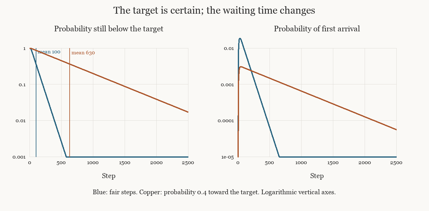
The left panel follows the fraction of unfinished experiments. The right panel shows the probability of first arrival at each allowed step; only steps with the same parity as the target can contain an arrival. Both models eventually reach the target, but the drift toward the reflecting wall leaves a much longer survival tail. The vertical marks indicate the exact mean waiting times, obtained from the backward equation rather than estimated from the plotted interval.
The target is rare here because the typical local tendency points away from it. A successful excursion must accumulate an unusual excess of rightward steps before returning to the wall. Increasing asks this imbalance to persist over a longer excursion. The probability cost is multiplicative, which appears as exponential growth of the mean waiting time. The exponent and prefactor belong to this discrete model and its boundary rule; they are not a universal formula for every barrier-crossing process.
Typical time and mean time
A mean waiting time does not say that most trajectories finish near that value. For the fair walk to ten, half of the experiments finish by step 76, while the mean is one hundred. For the biased walk, half finish by step 442 while the mean is approximately 630. The survival tail pulls each mean above its median. The means follow from the exact recurrence; the medians come from propagating its probabilities until cumulative arrival reaches one half.
The distinction becomes sharper for an unbounded fair walk with a target on only one side. Take the nearest target, one step to the right of the starting point. A first arrival on step requires the walk to remain at or below its starting point for the preceding steps. Counting these paths gives
The symbol in parentheses is a binomial coefficient, the number of ways to choose objects from ; the additional factor selects paths that have not crossed the target earlier. For large , this probability decreases in proportion to . Its sum over all is one, so the target is eventually reached with probability one. Multiplying by the arrival time to calculate the mean leaves terms proportional to , whose sum does not settle to a finite value. Most trajectories arrive in finite time, while increasingly rare and long excursions keep changing the average. Certainty of eventual arrival and existence of a finite characteristic waiting time are separate properties.
This is also why an empirical average can be unstable. If the waiting-time distribution has a long tail, a new observation can change the sample mean substantially even after many completed experiments. Reporting a mean alone hides both the fraction that has completed by a practical deadline and the uncertainty caused by the tail. A survival curve, selected quantiles and the observation window reveal different parts of the process.
The hazard at step asks a conditional question: among trajectories that survived through step , what fraction arrive on step ? It is when the denominator is positive. A decreasing survival curve does not imply a constant hazard. Treating rare events as if they arrived with a fixed rate requires another model and another assumption about memory.
What an observed crossing can establish
Suppose we watch a physical system escape from a region and record the first crossing of a threshold. The threshold must specify an observable and a direction of crossing. Measurement resolution matters: a coarse sampling interval can miss a brief crossing and report a later one. Resetting the experiment after each event must also reproduce the intended initial condition; otherwise successive waiting times need not share one distribution.
Our finite walk predicts the entire survival curve once , the boundaries and the starting position are fixed. We can test more than its mean. Changing the target distance distinguishes quadratic growth from the exponential dependence produced by a drift away from the target. Changing the starting position tests the backward relation between neighbouring states. Comparing first-arrival probabilities tests whether the tail and the parity structure agree with the proposed stepping rule.
Real barrier crossing may involve continuous motion, thermal noise, a varying drift or hidden degrees of freedom. Gardiner's Fokker–Planck treatment expresses the same first-passage logic for continuous diffusions: absorbing boundaries remove probability, survival is the remaining probability inside the region, and the mean solves a backward equation with boundary conditions. The coefficients of that equation encode the physical drift and fluctuations. Inferring them from waiting times alone can be underdetermined, since different mechanisms may produce similar means while predicting different survival curves or responses to intervention.
The first crossing turns a trajectory into a duration. Its distribution depends on the motion throughout the allowed region and on what happens at its boundaries. A rare event can therefore reveal dynamics that ordinary fluctuations near a frequently visited state scarcely probe—but only if we retain when the event occurred, how the experiment was prepared and which paths were still unfinished when observation stopped.
Letture collegate