How does a system recover?
Water enters a tank through a pipe and leaves through a controlled outlet. The volume in the tank is a stock, an amount accumulated at a particular moment; the incoming and outgoing flows are rates, measured in litres per minute. If two litres enter each minute and one litre leaves, the volume initially increases at one litre per minute. A level reading gives the amount present, while measurements of the two flows tell us how that amount is changing. A large volume need not imply rapid filling, and a tank whose volume is constant can still have water passing through it continuously.
A balance of flows
To follow such a system, let denote the volume at time . The parentheses indicate that the value depends on time. Over an interval lasting half a minute, a net inflow of one litre per minute adds half a litre, provided the rate stays unchanged throughout that interval. If the rate itself varies as the tank fills, we can shorten the interval until its variation is small, estimate the volume gained or lost, and repeat using the newly reached volume. This is how a rule for a rate becomes a prediction for an evolving quantity.
The notation expresses the instantaneous rate of change. We obtain its meaning by comparing the change in volume with the duration of the observation and considering progressively shorter intervals. It is measured in litres per minute, whereas is measured in litres. Conservation of water, under the assumption that evaporation and other losses are absent, can then be written as
Here the two quantities on the right are the incoming and outgoing flow rates. The equation states the accounting rule. To use it, we must also specify how those flows are determined. An incoming pipe might provide a nearly constant supply, while an outlet might respond to the water level or to the setting of a pump. Different relations between flow and volume produce different dynamics even though the conservation equation remains unchanged.
How the return is produced
Consider a tank supplied at one litre per minute, with an outlet pump adjusted to remove one hundredth of the current volume per minute. At a volume of fifty litres it removes half a litre per minute; at one hundred litres it removes one litre per minute. We assume that its response is effectively immediate and that the pump operates within the range where this proportional rule can be maintained. This is a specified model of a controlled outlet, rather than a general law for water escaping through an ordinary hole.
At one hundred litres, inflow and outflow balance, so the volume stays constant. If we add ten litres, the outlet now removes 1.1 litres per minute while the supply remains one litre per minute. The excess starts to decrease. If instead we remove ten litres, the outlet removes only 0.9 litres per minute and the tank begins to refill. A disturbance changes the outflow in a direction that opposes the disturbance.
This dependence forms a negative feedback: increasing the stock increases a process that reduces it. The loop can be followed through the apparatus, from the volume reading to the pump setting and back to the volume. Its sign refers to the effect of a departure, so negative does not mean harmful. In this particular model the loop stabilizes the level because its response is immediate, proportional and unopposed by additional dynamics.
The constant volume is a fixed point of the evolution rule. If the model starts at that value, it remains there. Because nearby volumes return toward it after a small disturbance, this fixed point is also attracting and locally stable; the combination is often called asymptotic stability. The return toward it is a property of the rates around the fixed point, rather than of the mere fact that they cancel at the point itself.
A graph of net flow against volume makes the restoring tendency visible. Below one hundred litres, the net flow is positive and the volume increases; above it, the net flow is negative and the volume decreases. The zero of the curve locates the fixed point. This graph describes a rule for all initial volumes, whereas a graph of volume against time follows one preparation through its history.
For the chosen pump setting, an additional litre causes an additional outflow of 0.01 litres per minute. If we doubled the proportional response and also doubled the supply, the balanced volume would remain one hundred litres, but an excess would be removed more quickly. Locating a fixed point and determining its rate of recovery are separate parts of understanding the dynamics.
The time scale of recovery
For the original setting, call the excess above the balanced level . The net flow is then litres per minute. During a sufficiently short interval, the model removes the same fraction of the excess regardless of its current size. An excess of twenty litres initially shrinks twice as quickly as an excess of ten, but it also has twice as much distance to recover. This repeated loss of a fraction produces exponential decay.
We can understand the exponential through the short-interval construction. Approximating the motion in one-minute steps multiplies the excess by 0.99 at each step. Using half-minute steps instead multiplies it by 0.995 twice per minute. Shortening the steps further follows the continuously adjusting pump more accurately. Over one hundred minutes, the remaining fraction approaches approximately 0.368. This number is conventionally written , where is about 2.718. Over two such intervals the fraction is , because the same reduction is applied twice.
The relaxation time is the interval over which an exponentially decaying excess is multiplied by . For this tank it is one hundred minutes. Its role can be recorded as
The initial excess is , and the ratio counts how many relaxation times have passed. The exponent must be dimensionless, which is why a time is divided by another time. After approximately 69.3 minutes, the remaining excess is half its initial value; after one hundred minutes, about 36.8 per cent remains.
A stable volume in this tank is maintained by a continuous throughput. Calling it an equilibrium solution of a dynamical equation means that the variable in that equation remains constant. It does not establish thermodynamic equilibrium of the apparatus, since a supply and a powered pump continue to operate. The physical processes supporting a fixed value remain relevant even when the value itself is unchanged.
More than one destination
Within the operating range where the proportional pump rule remains valid, a disturbance on either side of one hundred litres returns toward that level. Other rules can admit more than one long-term outcome. To understand what then selects the outcome, consider a population whose members reproduce poorly when very few are present because encounters between potential mates are scarce. At intermediate abundance, reproduction becomes easier; at high abundance, competition for limited resources reduces the net growth again. The population influences the conditions of its own increase.
We can describe the resulting possibilities using an illustrative rule. Let the net growth vanish at population sizes zero, twenty and eighty. Suppose it is negative between zero and twenty, positive between twenty and eighty, and negative above eighty. The numbers are chosen for the example and do not represent observations of a particular species. Immigration is excluded, the environment is held fixed, and population size is treated as a continuous variable, which can approximate many individuals but loses the discreteness that matters near extinction.
One smooth equation with these properties is
where is population size and is a positive rate setting the time scale. The factor makes the growth rate zero when nobody is present. The middle factor changes sign at the threshold , while the last changes sign at , the upper balanced population. Below twenty, the middle factor is negative and the last is positive, so their product gives a decrease. Between twenty and eighty both are positive, so the population grows. Above eighty, the last is negative and the population decreases. Reading the signs is enough to reconstruct the directions of motion.
This is a model of a strong Allee effect, in which sufficiently low abundance leads to negative net growth. The chosen product is a convenient way to encode the assumed dependence; explaining a particular population would require evidence for that dependence and estimates of its parameters. Finding the same shape of curve in two contexts would not establish that encounters between mates are the mechanism in both.
In the deterministic model, an initial population of thirty grows toward eighty, while one of ten declines toward zero. The continuous model approaches extinction as a limit; an actual population consists of whole individuals, and its final losses require a discrete description. The threshold at twenty is itself a fixed point, but a small displacement from it grows: moving just below it starts a decline, while moving just above it starts growth toward eighty. The threshold therefore repels nearby trajectories. At eighty, departures on either side bring the population back, so that fixed point attracts nearby trajectories.
The boundary of recovery
The collection of starting states that approach a particular attractor is its basin of attraction. Here initial populations from zero up to, but excluding, twenty approach zero, while those above twenty approach eighty. The boundary is the unstable state at twenty. A population near eighty can recover from many disturbances, yet a sufficiently large loss can carry it across that boundary and lead to a different outcome even though the environmental parameters have not changed.
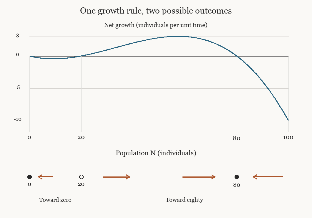
The upper curve is the specified growth rule with per unit time, and . The arrows below it show the direction of change. Filled points attract nearby states in the physical domain ; the open point at twenty separates the two basins. The curve is an illustrative model, with no fit to biological data.
The strength of local recovery and the size of the basin answer different questions. A rapid return after a small disturbance gives information about the nearby growth curve. It leaves open how large a disturbance would carry the system beyond the basin boundary. In the population example, changing the overall rate speeds up or slows down the entire motion while leaving the threshold and the basins in place. The speed of recovery alone therefore cannot determine the size of the disturbance that changes the eventual outcome.
These conclusions concern disturbances to the state while the rules remain fixed. A change in the environment can move the threshold itself; immigration can remove the absorbing condition at zero; fluctuations can carry a population across a boundary that a deterministic trajectory never crosses. The basin gives a precise answer within a specified model. Applying that answer to a living population requires deciding which of these processes can be neglected on the time scale of interest.
An observation of recovery is therefore evidence about a particular neighbourhood of the state being observed. To learn what lies farther away, we need information about the growth or flow rule beyond that neighbourhood. Measuring how quickly a small disturbance decays and determining which disturbances change the eventual outcome are distinct experimental tasks.
Letture collegate