What do we need to know?
A photograph of a swinging pendulum leaves something unresolved. The bob may be passing through the centre of its swing from left to right, or it may be passing through the same position in the opposite direction. Those two moments can produce the same photograph and have different immediate futures. Even knowing the position very accurately will not tell us which way the bob is moving. The missing quantity is its velocity.
If the same recorded state admits different future evolutions under the same deterministic rules, we should ask whether relevant information has been omitted. For a simple mechanical system, position and velocity can supply that information together.
A state with two coordinates
Consider a small glider moving along a horizontal rail, attached to a spring. We measure its displacement from the position where the spring exerts no horizontal force. A positive value places the glider to the right of that position, and a negative value places it to the left. The velocity is positive when the glider moves right and negative when it moves left. A positive displacement can therefore coexist with either sign of velocity: the glider may be moving farther from the centre or returning toward it.
Suppose we pull the glider to the right and release it from rest. The stretched spring pulls it toward the centre. Its velocity becomes negative, and the glider starts moving left. As the spring approaches its relaxed length, its force diminishes, but the velocity accumulated during the approach remains. By the time the glider reaches the centre it is already moving, so it passes through. The force now points to the right and slows its leftward motion until it stops at the other end of the swing and begins to return.
We can represent the additional information by giving the state space a second axis. Let horizontal position in the drawing record the displacement , and vertical position record the velocity . A point on this plane specifies both quantities at once. The glider still travels along a one-dimensional rail in the laboratory; the second direction in the drawing represents a second variable in its description.
On the horizontal axis, velocity is zero: the glider is instantaneously at rest even if its spring is stretched. On the vertical axis, displacement is zero: it is crossing the centre unless velocity is also zero. Only the origin describes rest at the relaxed spring position.
Within a range where a spring behaves approximately linearly, its restoring force is : proportional to displacement and directed toward the centre. The positive constant measures stiffness. This proportionality is an assumption supported by measurement over an appropriate range; a real spring can depart from it at large deformations.
Newton's equation relates net force to the rate of change of momentum. For constant mass , momentum is , so acceleration equals force divided by mass. Neglecting friction, we obtain
The notation expresses how rapidly position changes at an instant. Its meaning comes from measuring displacement over a short interval, dividing by the duration, and considering progressively shorter intervals. The notation applies the same procedure to velocity, giving acceleration. At any point , the equations specify both rates. Multiplying them by a short time interval gives an approximation to the next change of state.
Start to the right of the origin on the horizontal axis, where the glider has positive displacement and zero velocity. The state point initially moves downward: position is momentarily stationary while velocity becomes negative. It then moves left, crossing the vertical axis below the origin as the glider passes through the centre. At the leftmost point, velocity reaches zero and the glider turns back.
One circuit of the closed curve represents a complete oscillation. Its upper half describes motion to the right, its lower half motion to the left. Such a curve is a trajectory in phase space; drawing trajectories for several initial conditions gives a phase portrait.
What energy leaves unresolved
The closed curves have a physical explanation in the exchange between stored spring energy and kinetic energy. To stretch a linear spring from zero to displacement , an external agent must work against a force that rises from zero to . The work is force accumulated over distance. Since the force rises linearly, its average during that stretching is half its final value, and the stored energy is . Stretching or compressing gives a positive energy because the displacement is squared.
The kinetic energy can also be connected to work. Imagine accelerating a mass from rest with a constant force, giving it constant acceleration . To reach speed takes time , and its average speed during that interval is . The distance travelled is consequently . Multiplying by the force gives the work done, . In classical mechanics this is the kinetic energy associated with the resulting speed.
For the frictionless glider, the energy accounted for by these two contributions is
As the glider approaches the centre, stored spring energy becomes kinetic energy; after it crosses, the exchange reverses. No energy leaves the frictionless model, so the total stays constant and fixes one closed curve in the phase portrait.
Knowing the energy alone still leaves the position on that curve unresolved. A glider at rest with a stretched spring and one passing quickly through the centre can have the same energy and different immediate futures. Energy is an observable that groups states together. Its conservation restricts where the trajectory can go, without specifying the state occupied.
For a given value of , the largest displacement occurs when velocity is zero, while the largest speed occurs at zero displacement. The curve satisfying the energy equation is an ellipse on axes with general scales. In a numerical example with kilogram and newton per metre, plotting displacement in metres and velocity in metres per second gives circles, because the numerical coefficients of the two squared coordinates agree. Changing the units or the stiffness changes the shape drawn on the page without altering the interpretation of a closed orbit.
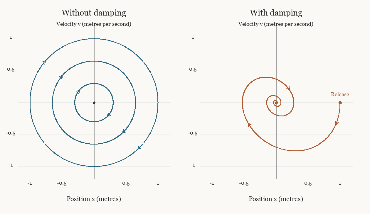
The left panel shows constant-energy trajectories for kilogram and newton per metre. The right adds resistance , with kilograms per second, starting at metre and .
When motion loses energy
The family of closed curves reveals a distinction within the language of stability. A small displacement of a glider initially at rest gives it a small amount of energy, and the subsequent oscillation stays near the origin. The origin is stable in the sense that sufficiently small disturbances remain small. It does not attract those disturbed trajectories, since their energy remains above zero and they continue circulating on their own closed curves. Returning toward an equilibrium and remaining near it are different properties.
This behaviour changes when we allow energy to leave the mechanical motion. Suppose the glider encounters a resistance proportional to velocity and opposing it, represented by the force , with . Such a law models linear damping within a suitable operating range. The equations become
Resistance opposes motion, although the glider can still gain speed when the spring’s contribution exceeds it. Multiplying force by velocity gives work per unit time. The damping contribution is , so mechanical energy decreases whenever the glider moves.
With weak damping, each excursion is smaller and the trajectory spirals toward the origin. The origin is now attracting as well as stable. In this smooth model the approach is asymptotic; an instrument may register rest before the mathematical limit is reached. Stronger damping can produce a return without repeated oscillations.
Trajectories cannot cross under these smooth autonomous rules: a shared position and velocity specify a unique evolution. A crossing in a plot of position alone may disappear when velocity is included, revealing the distinction hidden by the projection.
Autonomous means that the rule has no explicit dependence on external time. If a motor pulls the spring according to a schedule, predicting the force requires knowing the schedule’s current stage as well as position and velocity. This differs from comparing springs with different stiffnesses: those have different parameters and obey different rules. Whether a state is sufficient must be tested under the same specified rules.
A smaller description
A similar distinction applies when the rules themselves are probabilistic. Suppose we record the side of a container occupied by each of four particles, and at every turn choose a particle at random and assign it to either side with a fair coin. A complete record of the four assignments does not determine the next assignment with certainty, because the rule calls for new random choices. It does determine the probabilities of the possible next assignments. In a stochastic model, the relevant question is whether the proposed state supplies enough information to assign those probabilities, without needing an additional record of the past.
Sometimes a much shorter description passes that test. For this particular reassignment rule, knowing only the number on the left is enough to predict the probabilities for the next count. A decrease requires selecting one of the particles on the left and then assigning it to the right. Its probability is therefore . An increase has probability , and the count stays unchanged with probability one half. The identities of the particles do not enter these probabilities, because the rule treats all four in the same way. We can predict the evolution of the count without predicting the evolution of every label.
This reduction depends on the rule. Imagine instead that one particle is selected twice as often as each of the other three. The probability of choosing that particle is two fifths, and the probability for each other particle is one fifth. If exactly one particle is on the left, the chance of losing it at the next turn is one fifth when it is the frequently selected particle, but one tenth when it is any of the others. The same left-hand count now conceals different probabilities for its immediate future. To recover a sufficient description, we could record both the count and which side contains the frequently selected particle.
We may care only about a count, a temperature or an amount of energy, yet predicting that observable can require information it does not contain. Which microscopic distinctions can be discarded depends on the dynamics and the question being asked.
Testing the boundary
The boundary drawn around the system is another part of this decision. In the damped glider, the mechanical energy decreases because we have allowed it to pass into degrees of freedom that the two-variable description does not follow. Calling this energy dissipated does not mean that energy has ceased to be conserved in a larger physical description. The surroundings receive it, while our model retains only its effect on the motion through the damping force. If the surroundings heat up enough to change the resistance appreciably, a fixed value of the damping coefficient may cease to describe the experiment. Temperature, or another property of the surroundings, could then need to be included or modelled separately.
These are questions that an experiment can expose. Prepare the glider at the same measured position and velocity on repeated occasions, keeping the nominal spring and damping parameters fixed. If its subsequent motion varies systematically with an unrecorded condition, such as the temperature of the apparatus, the two-variable description has missed something relevant. Differences can also arise from measurement error or from fluctuations that should be represented probabilistically. Repeated trajectories alone do not tell us which explanation is right; controlled changes to the preparation can help distinguish them.