Does the system explore its possibilities?
A light can be on or off. Once every second, a computer draws a fresh random number and decides whether to switch it. The probability of switching is the same in either direction. We watch for a minute, then for an hour, recording the light at every tick of the clock. What fraction of the record should show it on?
Symmetry suggests one half. Yet a light that almost never switches might remain on throughout our observation. Another, programmed to switch at every tick, would spend half its time on while remaining perfectly predictable. Equal proportions can coexist with very different histories. To understand what a record tells us, we need the rule that generates it and the time over which we observe it.
A distribution that stays the same
Call the switching probability . At each step the light changes state with probability and keeps its current state with probability . The new random choice is independent of previous choices. Knowing the present state is therefore sufficient to assign probabilities to the next one: this is the Markov property. It does not mean that successive observations are independent. When switching is rare, seeing the light on makes it very likely that the next observation will also be on.
Imagine many independent copies of the experiment. Let be the probability that a copy is on at step . The copies that will be on one step later arrive by two routes: some were already on and stayed there; others were off and switched. Adding these mutually exclusive contributions gives
The probability moving from on to off is ; the reverse flow is . Their difference changes the amount of probability assigned to the on state. If more than half the copies are on, the outward flow is larger, and the excess decreases. The switching rule has no knowledge of the overall population. This restoring effect follows from there being more copies available to leave the more populated state.
At , the flows match. Half the copies remain on in probability at every later time, even though individual lights keep switching. The distribution assigning one half to each state is stationary: one update leaves it unchanged. Here the two opposing flows also balance separately, an instance of detailed balance. With more states, stationarity requires total inflow to equal total outflow at each state; separate pairs need not balance, because probability can circulate around a loop.
The stationary distribution alone tells us nothing about the value of . A light that switches roughly once every ten seconds and one that switches roughly once every thousand seconds both preserve the same equal proportions.
How much of the starting point remains?
Now start every light on. The probability initially equals one, and the excess above the stationary value is one half. Subtracting one half from both sides of the update rule gives
Every update multiplies the remaining excess by the same factor. Repeating the rule times therefore gives
For , the absolute value of the multiplier is less than one, so the excess tends to zero. When , the approach is gradual and stays on the same side of one half. When , switching is more likely than staying, and the excess changes sign at each step while shrinking. At , a single update produces equal probabilities, whatever the initial state.
To measure mixing, we ask how close the distribution has come to stationarity even from the least favourable starting state. In this two-state model the discrepancy is : it is the largest error we could make in the probability of any event by using the stationary distribution. For larger state spaces the corresponding measure is called total variation distance.
Choose a tolerance of one percentage point. With , the discrepancy falls below after eighteen steps. With , it takes 1,955 steps, more than half an hour at one step per second. The stationary probabilities are identical, while the time required to use them for a light started in a known state differs by two orders of magnitude.
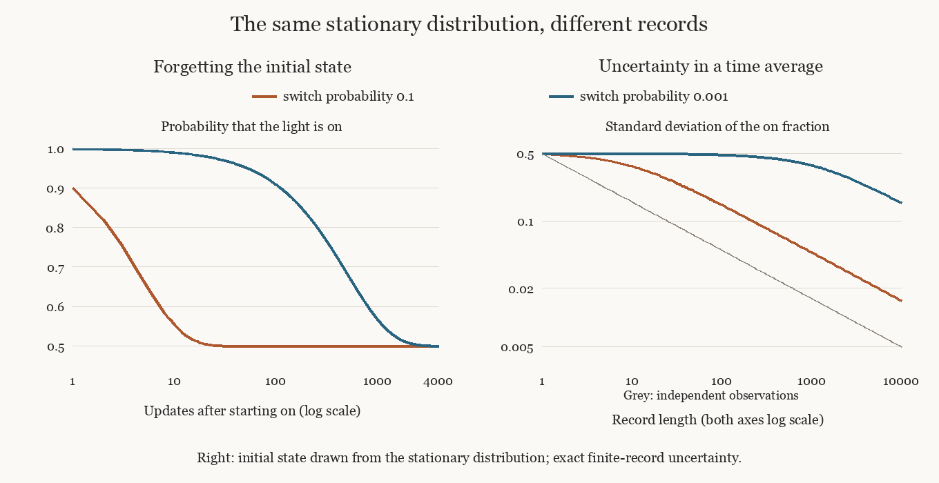
The left panel shows this loss of the initial imbalance. Both curves begin with every light on and approach the same horizontal line. The right panel concerns a different experiment: the initial state is already chosen with equal probabilities, and we measure the fraction of on observations along one record. Its uncertainty remains much greater for the slowly switching light. Starting with the correct distribution removes the initial bias; it does not remove correlations within a record.
For , the multiplier also gives a relaxation time: the number of steps that reduces the excess by a factor of is . For small , this is approximately . In the language of linear algebra, the multiplier is an eigenvalue, and its distance from one is the spectral gap of this model. An eigenvalue here says how much of a particular imbalance survives one update. In a larger chain, different imbalances can decay at different speeds; the slow ones can retain a memory of preparation long after faster changes have become invisible.
Visiting both states is not the same as forgetting
Two limiting rules reveal what the convergence argument needed. If , the light never switches. Every initial distribution is stationary, and each individual record stays in its starting state. There is no exchange between the two possibilities. The chain is reducible: its states fall into separate regions that cannot communicate.
At , every step switches the light. Both states are visited, and the equal distribution is the unique stationary one. Nevertheless, a light started on is certainly on at every even step and certainly off at every odd step. Its distribution never approaches one half. Returns to the starting state occur only at multiples of two; the chain is periodic.
The fraction of on observations along that alternating record does approach one half. Thus convergence of time averages and convergence of the distribution at a specified time are different claims. For a finite irreducible Markov chain, long-run visit frequencies converge to the stationary probabilities with probability one. Convergence of the distribution from every initial state additionally requires aperiodicity. Both properties are often gathered under the word ergodicity, so the precise claim matters more than the label.
Allowing a positive chance of staying put breaks the rigid alternation in our model. For any fixed , both states communicate and the distribution eventually forgets its initial condition. That statement places no useful upper limit on how long a finite experiment must run when is very small.
What a long record is worth
Suppose the light is initially on or off with equal probability. Write when it is on and otherwise. The fraction of on observations in a record of length is the average of through . Each observation has mean one half and variance one quarter, but nearby observations can repeat much of the same information.
The same update rule gives a correlation between observations steps apart of
For slow switching, knowing today's state remains informative about many subsequent readings. The variance of the recorded fraction must therefore include pairs of observations as well as individual ones. There are pairs separated by steps, giving
If observations were independent, only the first term in brackets would remain. For fixed and a record much longer than the correlation time, the bracket approaches . At , it approaches 999. A long record then carries, for estimating this particular fraction, roughly the precision of only independent observations. This approximation fails for short records; the right panel uses the finite sum instead.
This is a practical issue in Markov chain Monte Carlo. A computer generates successive configurations using a rule designed to preserve a desired distribution, then estimates an observable by averaging along the resulting history. The rule may be chosen for computational convenience, so its steps need not represent physical seconds. Preserving the target distribution is essential, but a slowly explored region can still dominate a finite calculation. Increasing the number of recorded steps helps according to the correlations they contain, rather than their count alone.
In the light model, the chance of seeing no switch in updates is . At , a thousand updates still have about a 37 percent chance of producing no switch at all. Such a record would look settled from beginning to end. Starting another light in the opposite state can expose the problem: two apparently stable records may disagree throughout the observation. In a larger model, agreement between a few runs is useful evidence, but it cannot rule out a region that all of them missed. The scientific question becomes which transitions have actually been sampled, and whether the quantities being measured have had time to lose their dependence on where the experiment began.