A path made of chance
Place a marker at the origin of a line. Every second, toss a fair coin and move the marker one millimetre to the right for heads or one millimetre to the left for tails. Each toss is independent of the previous ones. After a hundred moves, its position is the accumulated result of a hundred choices, none of which knew where the marker had already been.
Repeat the experiment and a different path appears. Some paths spend most of their time on one side; others repeatedly cross the origin. The average position over all possible repetitions is zero at every step, yet a typical marker does not remain at the origin. A theory that reports only this average leaves most of the motion unexplained. We need to follow the changing distribution of possible positions.
Following possibilities through time
After one toss, half the probability is at plus one millimetre and half at minus one. After two, the marker can be at minus two, zero or plus two millimetres. There are two ways to return to zero, right then left or left then right, and only one way to reach each outer position. Their probabilities are therefore one quarter, one half and one quarter.
Let be the probability of being at lattice position after steps. The index counts millimetres from the origin in our example. To arrive at on the next step, the marker must come from by moving right or from by moving left. These possibilities are mutually exclusive, so we add their probabilities:
The rule contains no uncertainty about how the probabilities themselves update. Given the current distribution, it determines the next one exactly. It does not determine which branch a particular marker will take. We have exchanged a prediction of an individual outcome for a prediction of the relative frequencies expected across repeated preparations.
Probability is conserved under this update. Every location sends half of its probability to each neighbour, so adding over all destinations recovers the full amount present before the move. There is no creation or disappearance of probability. Nor is there a restoring feedback toward the origin: the transition probabilities are the same everywhere. The growing spread results from accumulating independent steps, without any preference for returning to the starting point.
How far the marker travels
After a hundred one-millimetre moves, the marker has travelled a total path length of one hundred millimetres. Its displacement, the difference between final and initial positions, is usually much smaller. Leftward and rightward moves cancel in the displacement but both contribute to the distance travelled.
Call the step length . Each signed step has mean zero and variance , because squaring either or gives the same result. Independence makes the mean product of two distinct steps zero. Expanding the square of their sum therefore leaves one contribution for every step, giving
The angle brackets mean an average over repetitions, and the root-mean-square displacement is the square root of that average squared displacement. Since the mean displacement is zero, it also equals the standard deviation of position. After a hundred steps of one millimetre, it is ten millimetres. This is a measure of the spread, not a distance that every marker reaches.
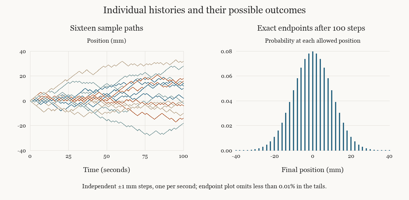
The paths on the left are sixteen realizations of the same rule. The distribution on the right is calculated from all possible hundred-step histories, rather than estimated from those sixteen paths. Its highest probability is at zero, but only about eight per cent of repetitions end there. The mean remains zero while most markers finish elsewhere. After an even number of steps, only even lattice positions are accessible; the stems preserve this detail of the discrete model.
If steps are separated by a time interval , then . It is convenient to define a diffusion coefficient
The coefficient has units of length squared per time. With our millimetre steps every second, is half a square millimetre per second. Multiplying elapsed time by four doubles the root-mean-square displacement. This differs from steady motion at a fixed velocity, where displacement is proportional to time. The relation estimates the time scale needed to spread over a distance; it does not give the mean time for first reaching a particular target, which depends on the target and the boundaries.
From a lattice to a density
At sufficiently coarse resolution, we may no longer distinguish individual lattice sites or single tosses. We describe the position by a smooth probability density . Density is probability per unit length: multiplying it by a short interval's width approximates the probability of finding the marker in that interval. The total area under the density is one. A density's value at one point is not itself the probability of that exact position.
To obtain such a description, we must average over the fine lattice structure. In particular, the alternating accessibility of even and odd sites in our walk cannot be reproduced by a smooth curve at every site. The approximation concerns intervals broad compared with the step length and evolution over many steps. Alternatively, a mathematical limit can shrink and together while holding fixed. The broad, slowly varying description then has a definite diffusion coefficient.
The discrete update can be rearranged as
The left side measures change in time. The right side compares a location's probability with the average of its two neighbours. At a local peak it is negative, so probability there decreases; at a local trough it is positive. This difference is a discrete measure of curvature. Dividing by the time step on the left and recognizing the spatial difference divided by on the right gives, for a smooth density,
The partial derivative on the left means the rate of change at a fixed location. The second spatial derivative on the right measures how the slope of the density changes with position. This is the diffusion equation. It follows here from local probability transfer and a controlled change of resolution. The equation describes the density; its smoothness does not make the underlying random path smooth.
Starting from a sharply localized position on an unbounded line, the continuum density is Gaussian at positive times, with variance . The peak lowers as the distribution broadens, preserving the total area. This bell is related to the central limit theorem: the position is a sum of independent finite-variance steps. The diffusion equation adds the temporal relation between the distributions at successive times.
A current without a preferred direction
There is a physical reason that symmetric steps can still produce transport from a crowded region toward a sparse one. Imagine many independent markers. At a boundary between two neighbouring sites, half the markers on either side move across in each update on average. If one side contains more markers, it sends more across even though each marker uses the same unbiased rule. The imbalance in numbers creates a net current.
For a smooth density, the resulting current is
A positive spatial slope means density increases toward the right; the minus sign makes the net current point left, toward lower density. This is Fick's law for the present homogeneous model. Combining it with conservation, which says that a region gains probability when more enters than leaves, reproduces the diffusion equation.
The same calculation can describe an expected particle concentration if many noninteracting particles follow the rule. The normalization then counts particles instead of total probability one. Inferring a smooth concentration from a single physical sample additionally requires enough particles in each observed region. Near-empty regions can have large relative fluctuations even when the equation for the expected concentration is accurate.
Which parts of a real motion survive?
A dissolved molecule does not literally wait for a clock to toss a coin. On short time scales its velocity has inertia and collisions have structure. A random-walk description becomes useful on scales where the relevant memory of those details is sufficiently short. The step variance and the rate of stepping then determine the diffusion coefficient in the idealized model; for a real material that coefficient must be derived from a suitable microscopic description or measured.
One can test this reduction by measuring how the mean-square displacement changes with elapsed time, examining the displacement distribution, and checking whether successive increments remain correlated. Persistent motion can produce an approximately quadratic mean-square displacement at short times before a linear regime emerges. A bulk flow adds drift; trapping can prolong waiting times; exceptionally long jumps can invalidate finite-variance assumptions. A linear mean-square displacement alone does not prove that every feature of the process obeys our independent-step model.
Boundaries change the question too. Reflecting walls retain probability and can eventually stop the spread from growing. An absorbing boundary removes trajectories when they first reach it, so the remaining probability measures survival. The free walk on an unbounded line has no such stationary confinement. Before using its diffusion coefficient to predict transport across a sample, we need to specify what particles do at the sample's edges. The local stepping rule and the boundary rule together determine the experiment we are describing.